RNNs a walkthrough
← back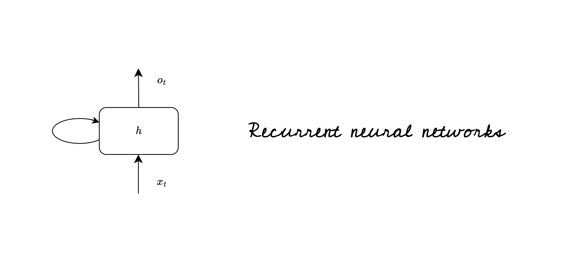
Contents
Introduction
Looking back from a point where GPT models have sent waves across the industry, recurrent networks have been one of the most fundamental blocks that have been laid down, when it comes to progress of natural language and deep learning. This blog aims to give a functional understanding of RNNs. Personally, I had a difficult time wrapping my head around this when i learnt it the first time. I believe that this blog would reduce the friction for the people who have just started their journey.
This blog is first in the series of Recurrent neural networks, LSTMs are extension of RNNs and we will go through a brief overview of RNNs first and understand their working and significance.
Why do we have recurrent networks?
Before jumping into a space of recurrent networks let us try to understand why do we need them in the first place?
Reason 1
For instance, you are a mobile phone’s keyboard that suggests a next word to a user. What would you try to learn in this case?
- Is the person frequently using a group of words?
- “This seems interesting”
- “Woah that’s awesome”
- How is a person talking to his friends or colleagues.
- “Hey, i am free tonight, lets catchup for games”
- “Hi, let us set up a meeting tomorrow morning”
- Is the sequence of some words same most of the time?
Notice how each word before gaming is setting up the context. You could suggest these words:
- Hey, i am free tonight, lets catchup for [games | walk | drinks]
- Hi, let us set up a meeting tomorrow [morning | afternoon | evening]
In order to give these word suggestions, you will have to remember these sequences, or to be specific the meaning that they convey.
Traditional neural networks are forgetful in nature, consider you are pass a sentence - “Hello are you free tomorrow evening” and you are passing this sentence word by word, by the time you pass the word “tomorrow” the network might have forgotten what words came prior to it. The network might learn which words occur most frequently with word tomorrow instead. Consider these sentences.
- “Tomorrow I have a meeting”
- “Tomorrow I have a holiday”
- “Tomorrow I won’t be available”
:bulb: Notice how using the word “Tomorrow” at the beginning and in between the sentence changes the next word prediction.
Say this is a general pattern for a person and his usage of word “Tomorrow”, if we use traditional neural networks we might suggest word “I” for the sentence “Hi, let us set up a meeting tomorrow ____”
Reason 2
We saw that we were not able to retain words using traditional neural networks, one might argue what happens if we show all words of sentence to neural network at the same time?
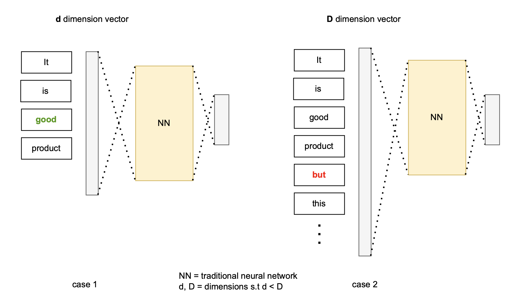
Say you want to classify text into 3 sentiments - positive, negative and neutral. And you are given a traditional neural network. Consider these 2 sentences.
- “It is a good product” → positive
- “It is a good product but it stopped working in few days” → negative
We can clearly see that each sentence has different number of words. It would hence change the dimensionality of vector representation for each sentence. If we truncate the sentence we lose meaning of the sentence, if we pad a sentence with dummy vectors we are increasing complexity of the network by increasing dimensionality.
To summarise we need a network which can:
- retain previously learnt information and build on top of that.
- handle sequences of variable length without increasing the dimensionality
Recurrent Network an overview
Some points to note before we begin this:
- Neural network is a computation unit
- Loop computation unit to get recurring neural networks
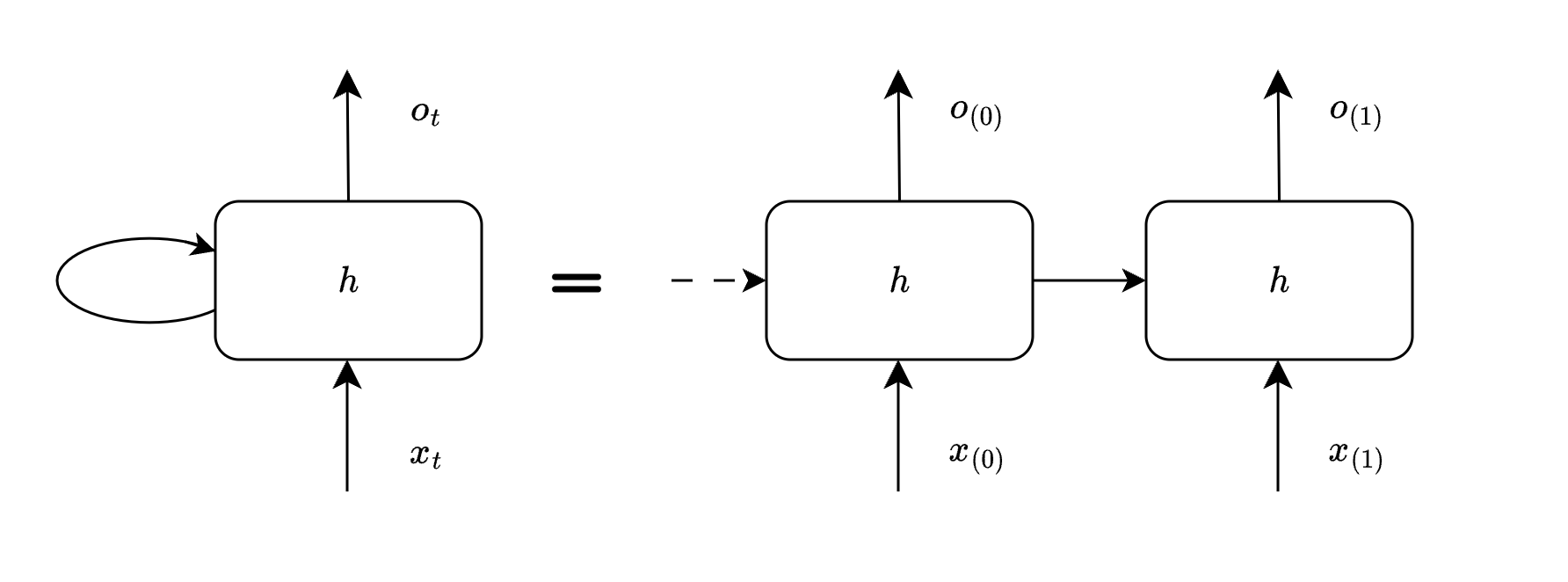
When you read about recurrent networks, this is a common diagram that you will stumble upon. Shown below is a simple recurrent cell.
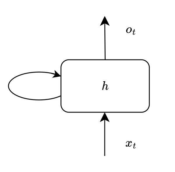
Let us call this recurrent unit as cell . Think of as a computation unit, it consumes some input and generates output . This cell is building block of recurrent neural network.
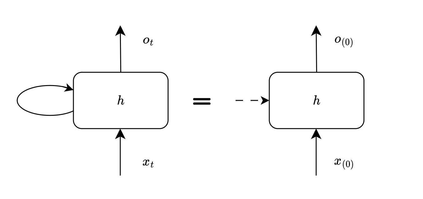
The loop shown above allows the network to carry previous information. Let us see how this network unrolls at each iteration (here iteration is called timestep). One thing to bear in mind before we proceed is that it is the same cell which we will be seeing at various timesteps.
t=0
At timestep 0 we do not have any previous information, hence a dotted line shown here indicates initialization of previous state.
t=1
At timestep 1 we do have previous information from timestep 0, we can consume this previous information to generate new output. For now let us not get into details as to what information is being passed, we will cover it in next section.
t=2
At timestep 2 we have previous information from timestep 1, we consume the same, and generate output in the similar way.
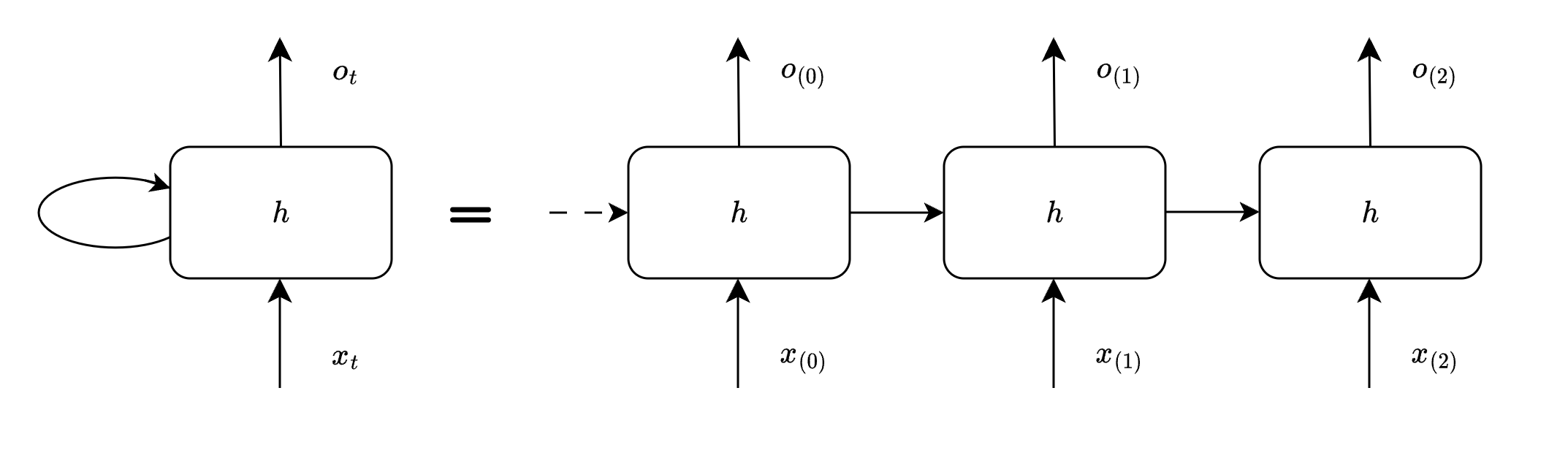
The same process continues for subsequent timesteps, until we run out of input.
Basic RNN cell
Now that we have some understanding of how information is being passed from previous states, let us look into detail to understand what hidden state actually does.
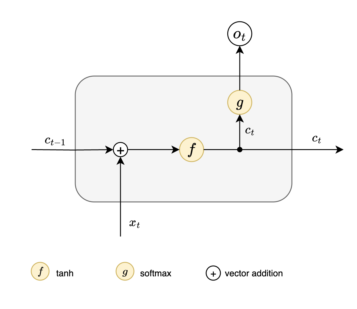
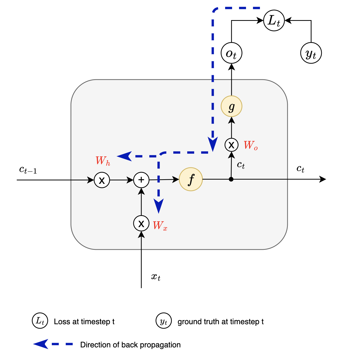
Simplified view of RNN cell
| = input at timestep t | = current cell state |
| = output at timestep t | = previous cell state |
Following steps occur when we pass input to RNN cell:
- Add previous cell state with current input
- This addition operation ensures that sequential dependencies are taken care of
- This is where we take into account previous hidden state
- Pass above output through non linear activation here tanh
- This nonlinearly activated output is called cell state
- Pass through here softmax to get current timestep output
- The same cell state will serve as previous state information for timestep
NOTE : At timestep RNN uses only cell state of , we do not have any information about states preceding .
Weights
This blog would be incomplete without a brief mention about weights involved in RNNs and how back propagation happens over each timestep.
There are 3 major weight matrices involved with RNNs. These weights are essentially what RNNs learn.
- - Input to Hidden Weights
- It determines how current input will influence the current cell state
- - Hidden to Hidden Weights
- It determines how previous cell state will influence current cell state
- - Hidden to Output Weights
- It determines the output based on current cell state
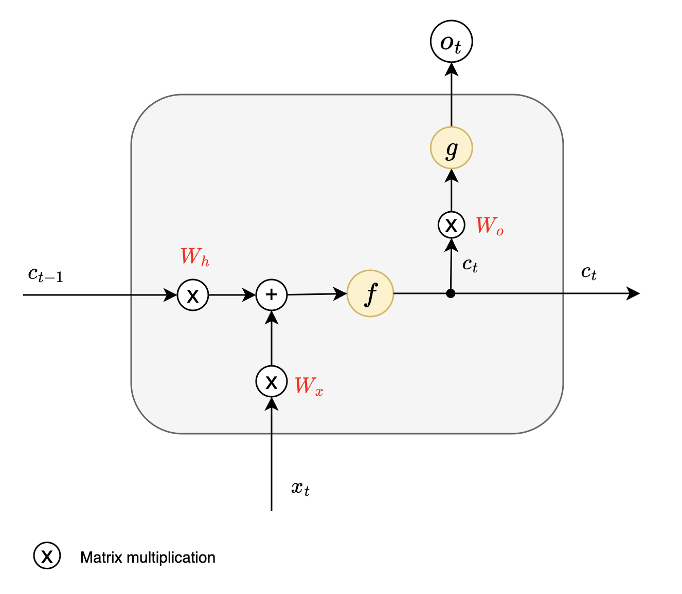
:bulb: Again it is worth noting that, same 3 weights are shared across all timesteps.
RNN can be represented using these equations
Where is tanh and is softmax activation.
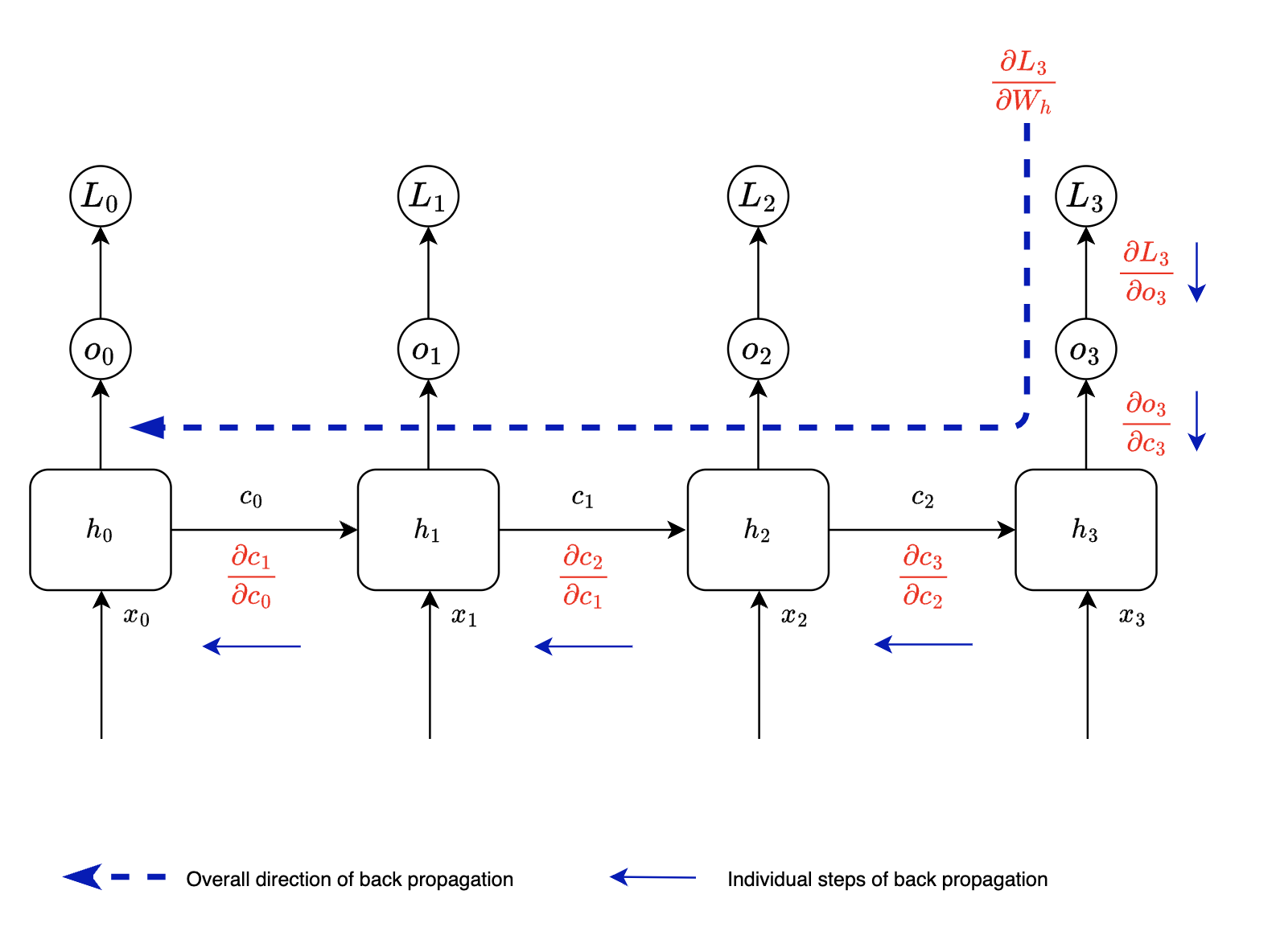
Back propagation through time
We will look at back propagation for one of the weights i.e the weight matrix associated with previous state. This is the most crucial set of parameters in case of RNNs.
Like any other back propagation we sum up individual losses. In case of RNNs we will sum up losses associated with each timestep and we will learn how these losses are varying with respect to weight matrices.
Let us look at term of
This is how RNN cell equations will look like at
We can write loss w.r.t as
Notice
- is dependent on
- is dependent on
Hence we need to apply chain rule of differentiation
If we extend the same observation
- is dependent on
- We can apply the same steps across for all timesteps
Hence we get following equation
Similar calculations will be done for in order to get
As we can see here BPTT (Back propagation through time) is nothing but sum of back propagations for each time step.
Limitations of RNNs
- Vanishing or exploding gradients
We saw how back propagation equation can be written for RNNs. Let us see how does it look for large sequences.
Notice how we are getting a long chain of multiplications
- if the gradients are smaller are between 0 and 1, it would lead to vanishing gradients
- if the gradients are greater than 1, gradients might explode
- RNNs are not able to learn long sequences
While RNNs are good at learning shorter sequences, their performance degrades with longer sequences. With longer sequences gradients tend to get smaller and hence hampers network’s ability to learn. This might result into very slow training.
References
- RNNs : Deep Learning Book by Aaron Courville, Ian Goodfellow, and Yoshua Bengio
- RNNs : Coursera Sequence Models
- BPTT : Backpropagation Through Time Overview - Sebastian Raschka
- BPTT : Backpropagation Through Time for Recurrent Neural Network - Mustafa Murat ARAT