LSTM simplified
← back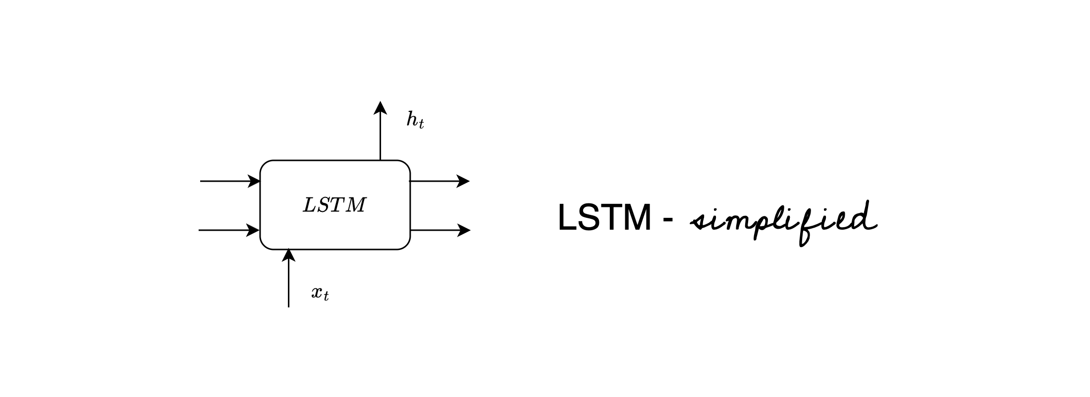
Contents
- 1. Introduction
- 2. The Gate
- 3. How do we concisely represent this “Gate”?
- 4. Some notations before we begin
- 5. Lego pieces
- 6. A Glimpse of an LSTM cell
- 7. A Math problem
- 8. Opening the Gates
- 8.1. Gate #1 - Forget Gate
- 8.2. Gate #2 - Input Gate
- 8.3. Gate #3 - Output Gate
- 9. The missing link
- 9.1. Case #1
- 9.2. Case #2
- 9.3. Case #3
- 9.4. Case #4
- 10. End note
- 11. References
Introduction
In my previous blog about RNNs - "RNNs a walkthrough", we saw how recurrent neural networks worked, their limitations, like vanishing gradients, which leads to failure of learning long sequences. LSTMs try to solve for these limitations. In this blog we will go through detailed walkthrough of underlying structure of an LSTM cell.
This is my effort to simplify each of the blocks of LSTM piece by piece. In the end we join all these pieces to answer the question - How is LSTM an add on over RNNs?
The Gate

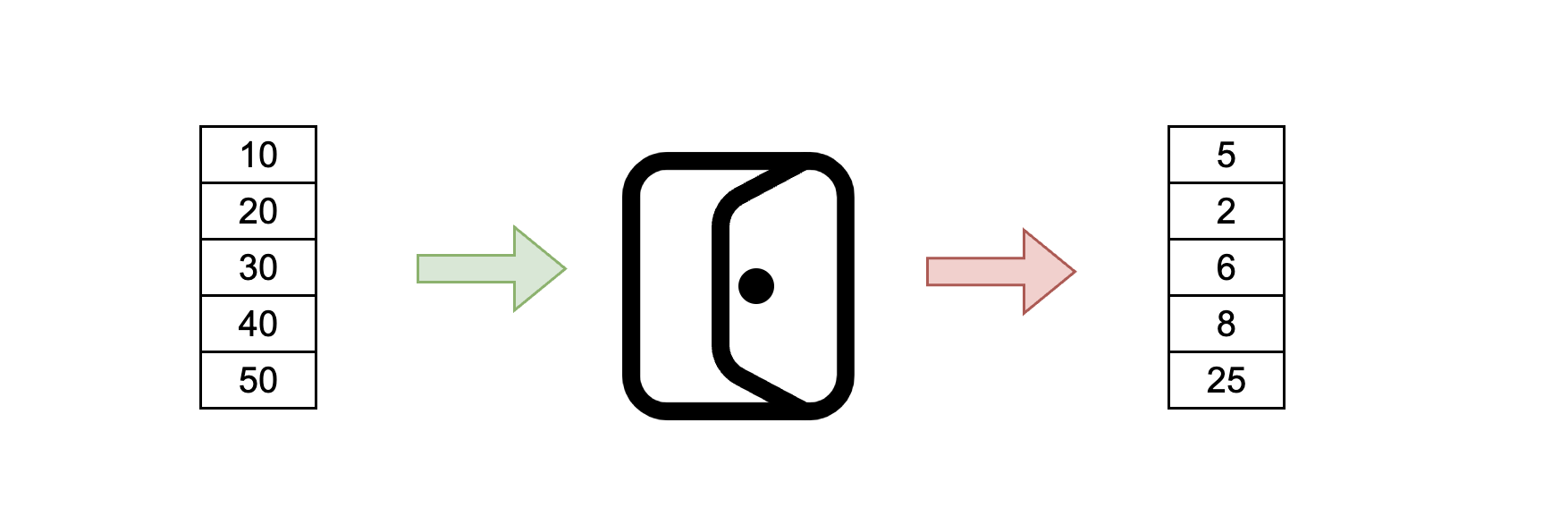
Believe me or not, the image above is the key to understanding the fundamental blocks of LSTM. This guard is protecting the gate above. For now let us assume that you will not be allowed through the gate without a small cost. Consider the same scenario with vectors. A vector cannot pass through certain path without a small cost. In the diagram below you can see that each value is reduced by some factor when it passes through the gate.
How do we mathematically achieve this? Simple, using a sigmoid layer. Range of Sigmoid function is between 0 and 1. (For now let us not worry about what is the input to this sigmoid layer)
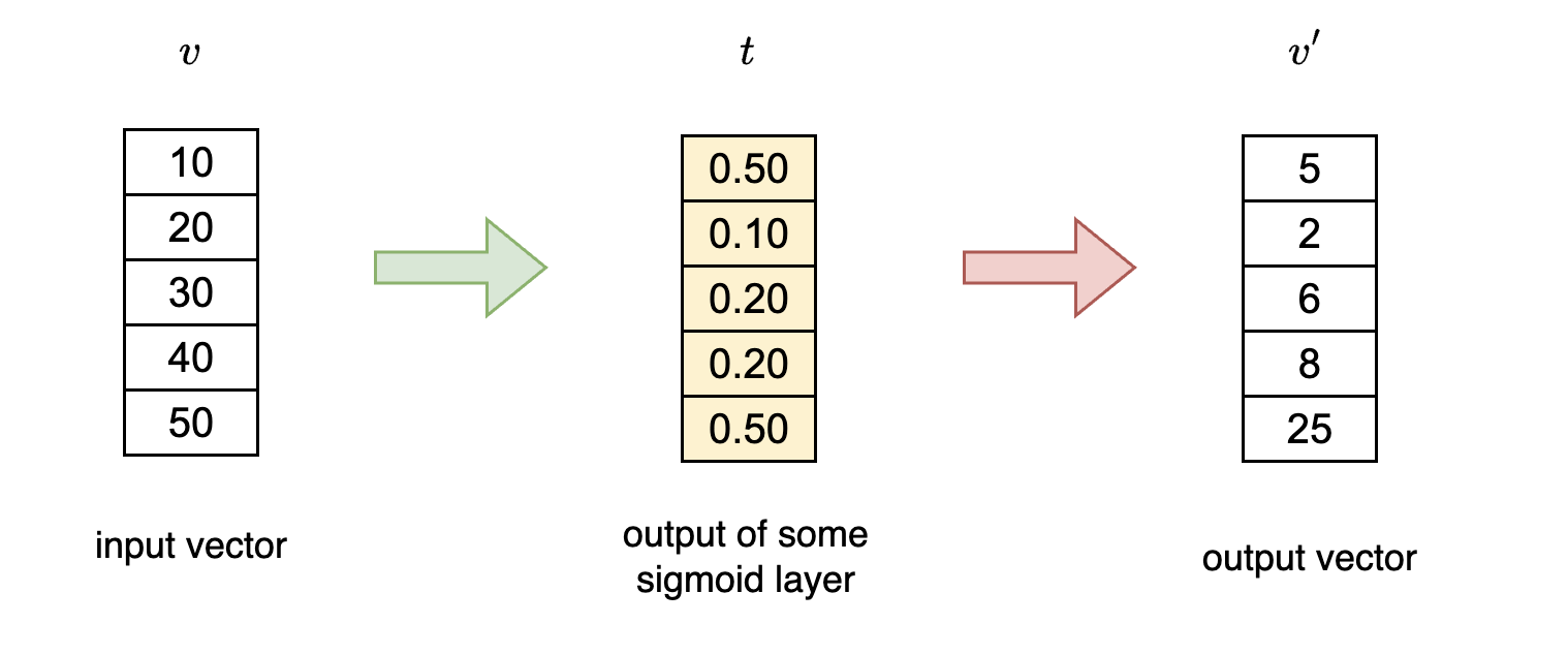
Notice how each element in the input vector is being multiplied with corresponding element in vector which is output of sigmoid layer to give resultant vector . This operation is called point wise operation. In this case we are performing point wise multiplication operation. This operation depicted above allows partial passage to the input vector.
What if we do not want input vector to pass through this special gate?
- Vector should be
[0,0,0,0,0]
What if we want input vector to pass without any change?
- Vector should be
[1,1,1,1,1]
How do we concisely represent this “Gate”?
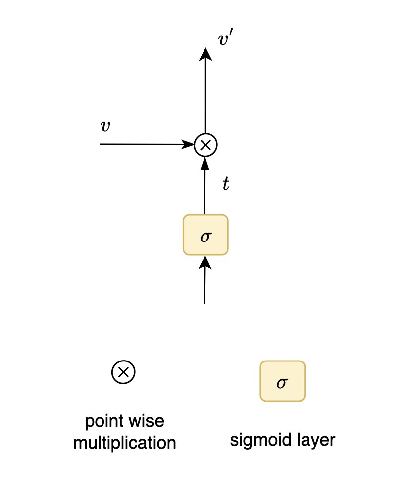
- vectors and have dimensions
- ⓧ here is the gate
- has elements in the range of 0 and 1 after sigmoid activation
- upon point wise multiplication a “fee” is collected to get new resultant vector
This procedure is critical to understand the gravity of the underlying structure of LSTMs, as this mechanism forms the basis of each fundamental block that we are going to discuss.
Some notations before we begin
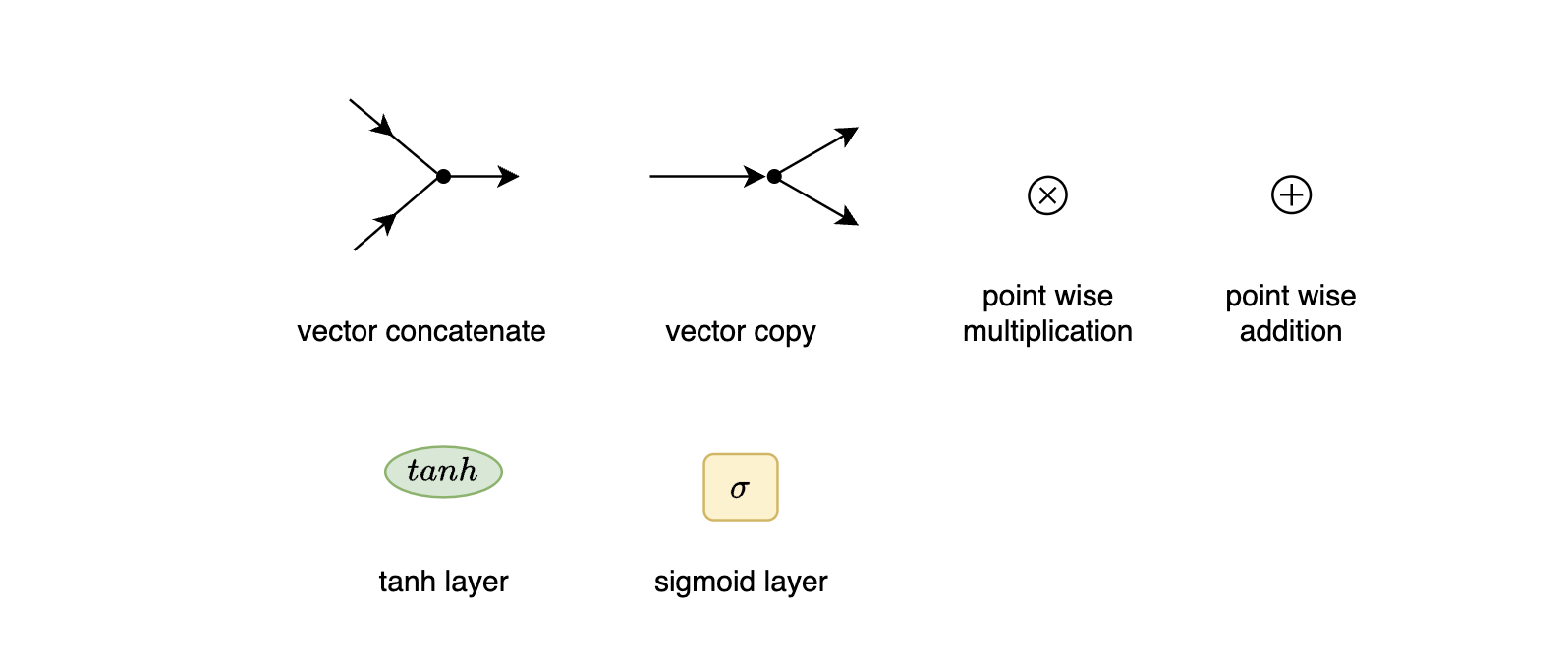
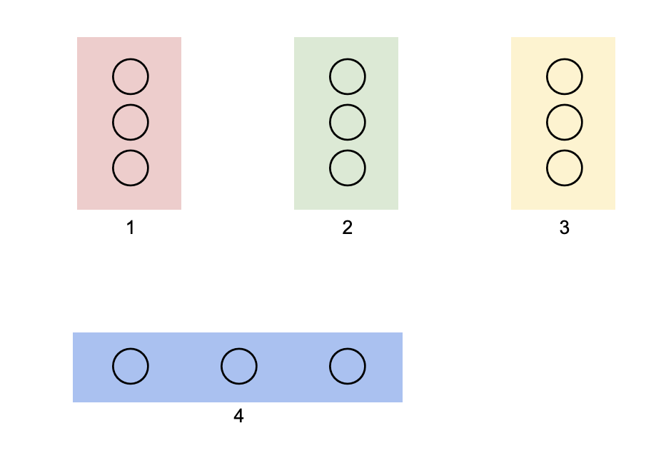
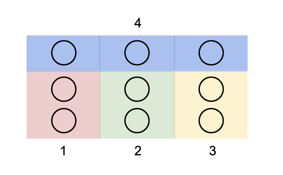
Lego pieces
An LSTM unit consists of 4 blocks, 3 blocks adjacent to each other and 1 block that connects them all each block has its own significance. In order to get an functional understanding let’s first look at each lego block individually, then we can club these pieces to form a complete LSTM unit.
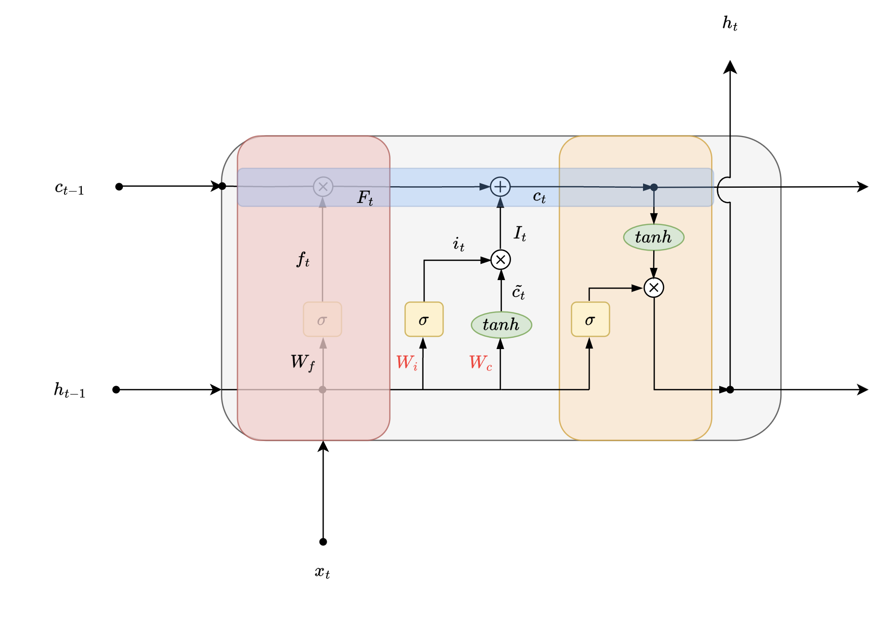
A Glimpse of an LSTM cell
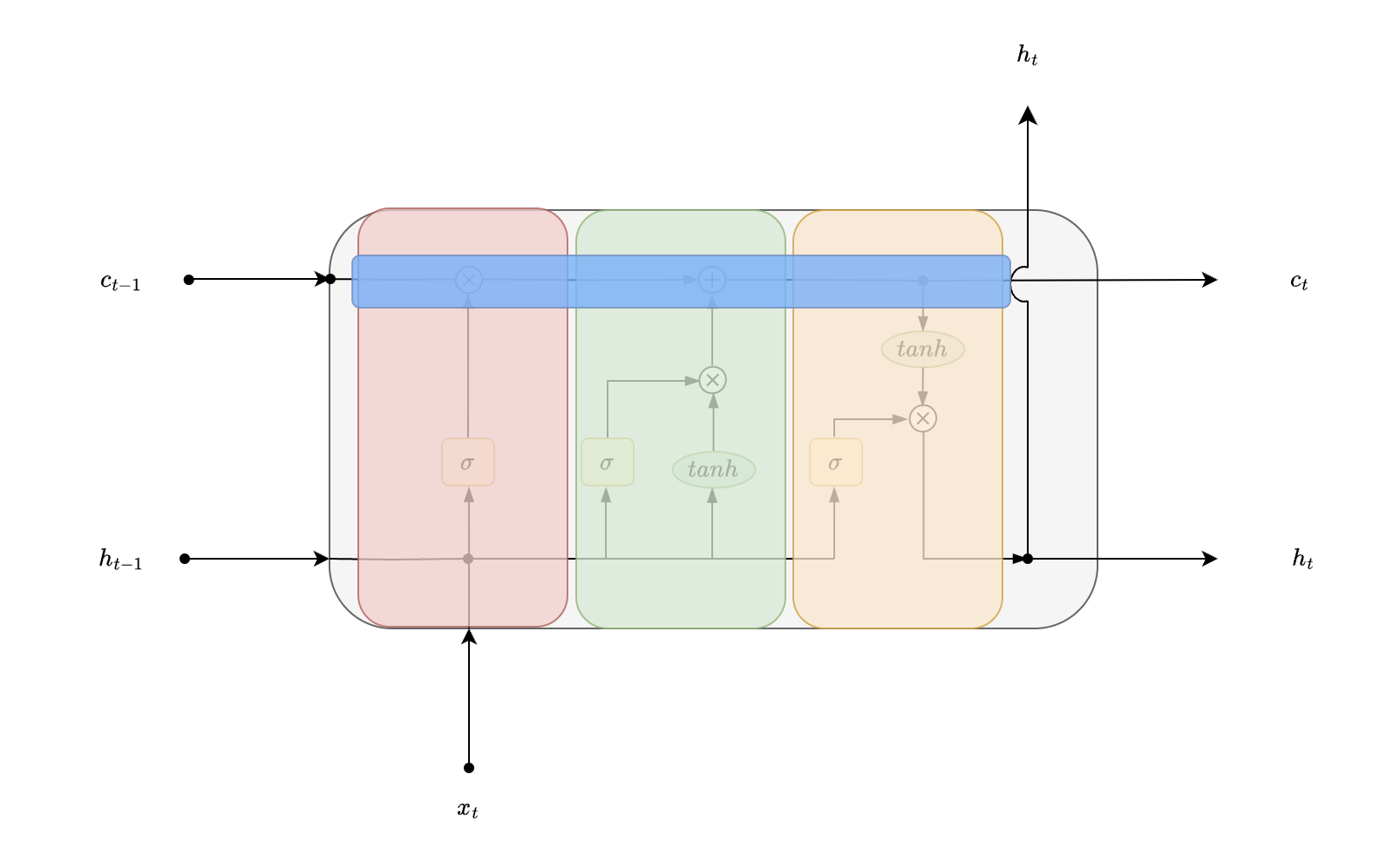
While LSTM cell is similar to vanilla RNN cell, one of the key distinction is that each state has 2 inputs from the previous time step, “cell state” and “hidden state” . All other concepts like unrolling a recurrent neural network, back propagation through time remain the same.
Unrolling LSTM cell for 3 timesteps - recursively consume outputs of previous state and current input to generate new state for current time step.
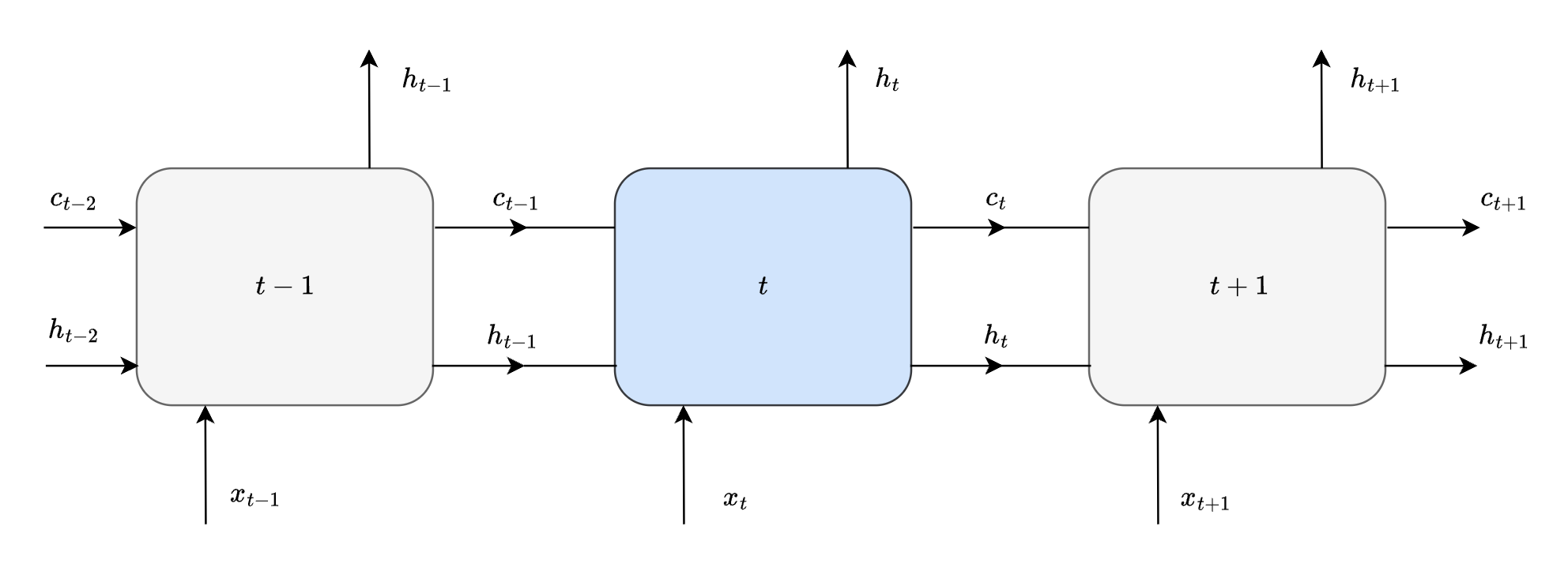
NOTE : it is the same LSTM cell that is being viewed at 3 time steps
A Math problem
I will be using a simple analogy to explain LSTMs. Consider you are in school and are being taught simple math.
Situation 1 - In classroom while learning you solve the problem:
- e.g - 10 apples cost 200Rs, what is the cost of 2 apples?
- Let us call this APPLE question
Situation 2 - In a test you are given a problem:
- e.g - 10 bananas cost 100Rs, what is the cost of 3 bananas?
- Let us call this BANANAS question
Steps to solve:
- cost of one object is
- cost of objects is
- solve for using given information
- find cost of objects using
💡 In order to solve a problem all that matters, is that you are able to recall the concept and use previously learnt steps to solve equivalent problem in future.
Though a trivial problem, it is important to list these steps down while trying to impose these steps on internal blocks of LSTMs.
Opening the Gates
Gate #1 - Forget Gate
What would your initial steps be while solving the BANANAS problem in exam?
- You retain the
- information you got from the new question
- for instance data mentioned in the bananas question
- You recall that
- you were taught to find cost of one apple
- you need to multiply cost of one apple with N apples in the question
- You forget the
- problem is about apples or bananas (It is actually about finding the cost of an object)
- answer to question you did in class (as it is not relevant for bananas problem)
Now let us impose this analogy on LSTMs.
| output of Forget gate | |
| weights associated with Forget gate | |
| bias associated with Forget gate | |
| sigmoid activated vector associated with forget gate | |
| concat vectors , | |
| previous hidden state | |
| previous cell state | |
| current input |
- retain
- input and previous time step output
- like data mentioned in the bananas question
- recall
- using cell state represents previous information that you learnt
- like steps to solve the problem
- forget
- some specifics partially which are not necessary, using the forget gate
- like is it apple or banana problem
It partially forgets previous and current information, here concatenated vector . Hence the name “Forget Gate”.
Now try to recall what we learnt in the earlier section about gates, it will cost you a certain fee to pass through. Same concept will be used here in order to “forget” information partially.
💡 But who decides what degree of information should be forgotten?
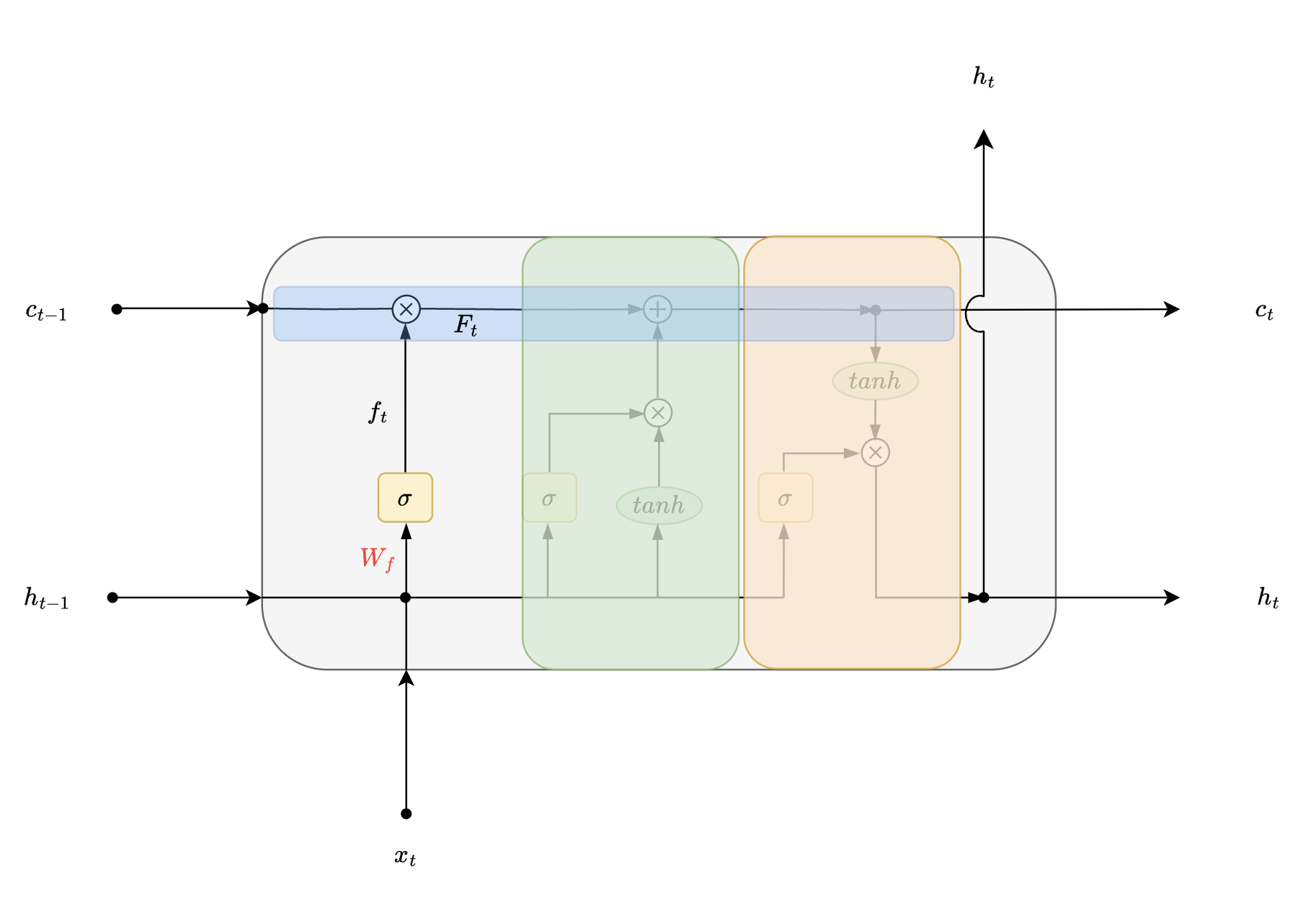
This is where weights and learning comes into play. Lets take a closer look at forget gate. Mathematically forget gate can be represented as:
- filter for “Forget Gate” - sigmoid activation
- output of “Forget Gate” - point wise multiplication
Notice how decision on degree of information that is to be forgotten is a function of 2 vectors and . We are forgetting previously learnt information partially on the basis of previous time step output as well as input of the current time step.
Now that we have passed through Gate #1 let us close it behind us and move to the next one.
Gate #2 - Input Gate
Again let us ask the same question now that you remember how to solve the problem, also you understand that it is a problem that involves calculating cost of single unit, what would your next step be?
- You recall that
- you need to setup a new equation based on new data
- this equation can be built using previous knowledge
- You set up
- a new equation to plug in values
- You forget the
- older equation (partially)
- values inserted in the older equation to solve apples question (completely)
Now let us try to see what LSTM does in this second stage.
| output of Forget gate | |
| output of Input gate | |
| weights associated with Input gate | |
| weights associated with Input gate | |
| sigmoid activated vector associated with input gate | |
| tanh activated vector associated with input gate |
- recall and retain
- input and previous time step output
- like recalling previous equation to solve apples problem and retaining bananas problem
- set up
- here activated vector can be a good representation of this step
- like coming up with equation for solving the bananas problem
- filter
- here point wise multiplication of and represents filtering
- like altering values inserted in the older equation to solve apples question
Very similar to “Forget Gate”, here LSTM tries to determine what degree of new information should be passed on to the next gate. This stage determines how to update old cell state of LSTM and by what amount. Weights which control Input gates are which help with filtering of input and which is associated with generating intermediate cell state of LSTM.
Mathematically it can be represented as
- create a filter for “Input gate”
- tanh activation for intermediate cell state generation of current time step
- Output of “Input gate”
Using the output of “Forget gate” and “Input gate” , a new state or a vector is formed called cell state. It essentially holds new information with some learnings from the past. Very much like us humans. We add new learnings on top of our knowledge bank while we retain our learnings from the past.
This cell state can be mathematically represented as
Notice how we are adding to previous knowledge using point wise operation here. This cell state is further used by “Output Gate” as well as the next timestep.
Gate #3 - Output Gate
Now we have the equation set up for us all we need to do is plug in the value and get the answer for our bananas problem.
- You retain
- values of bananas problem
- You solve
- for new answer according to bananas problem
- (using previously learnt concept like multiplication)
- You filter
- imagine you are required to just fill in the final answer into the test
- steps are not relevant here, so you filter that and report just the final answer
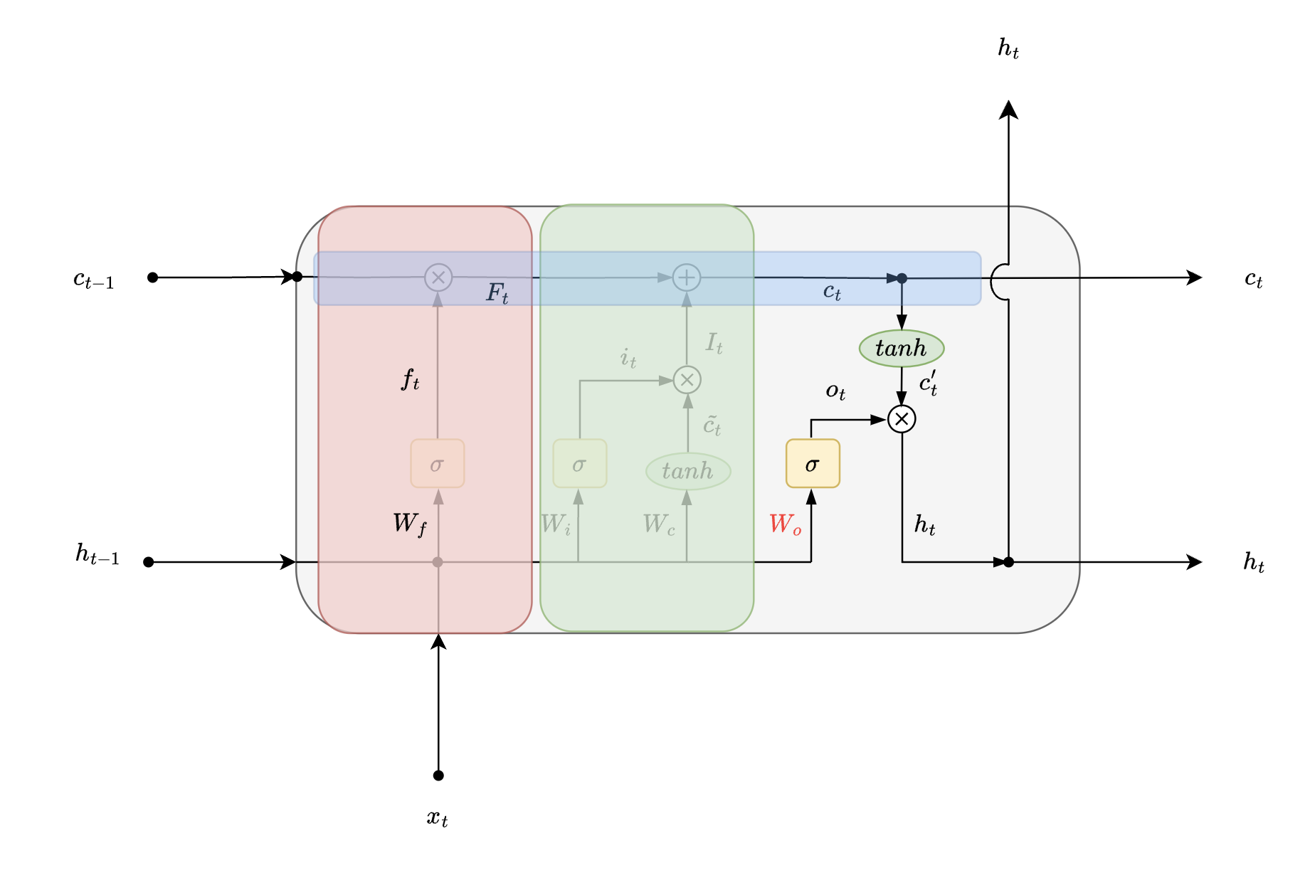
Let us look how LSTMs generate final output.
| weights associated with Output gate | |
| sigmoid activated vector associated with Output gate | |
| cell state associated with current time step | |
| tanh activated vector associated with Output gate | |
| hidden state output associated with current time step |
- recall and retain
- input and previous time step output → this step remains same
- like recalling previous method to get final answer and retaining bananas problem
- solve
- here activation of cell state is a good representation of process of getting the answer
- like solving for cost of n objects
- filter
- creating a filter similar to earlier gates here termed as
- filtering using to get which is the final output of current state
- like reporting just the final answer
The goal of this gate is to generate hidden state output associated with current time step. Filtering using sigmoid activation remains the same as seen in earlier gates, only the weights and biases associated with this gate change.
Mathematically this stage can be represented as:
- create a filter for “Output gate”
- tanh activation associated with “Output gate”
- output of “Output gate”
Notice how
- final output is function of transformed current cell state
- in earlier gates we saw that how is function of previous cell state and current cell state
- This happens in a recursive fashion just like vanilla RNNs
All these transformations are good but what exactly makes LSTM so special? For this we will need to ask ourselves how did LSTMs solve for issues which vanilla RNNs faced.
The missing link
In this section we will try to answer how does LSTM solve for “long term dependencies”. The easiest way to explain the piece that binds it all would be using how gates can be utilised in order to retain long term information.
For now we are concerned with two gates forget gate and input gate. Clearing rest of the paths in LSTM for ease of explaining.
Equations of LSTM at various timesteps
timestep = t
- Output of forget gate
- Output of input gate
These equations can be combined to get
Let us see the same set of equations at various timesteps
timestep = t+1
timestep = t
timestep = t-1
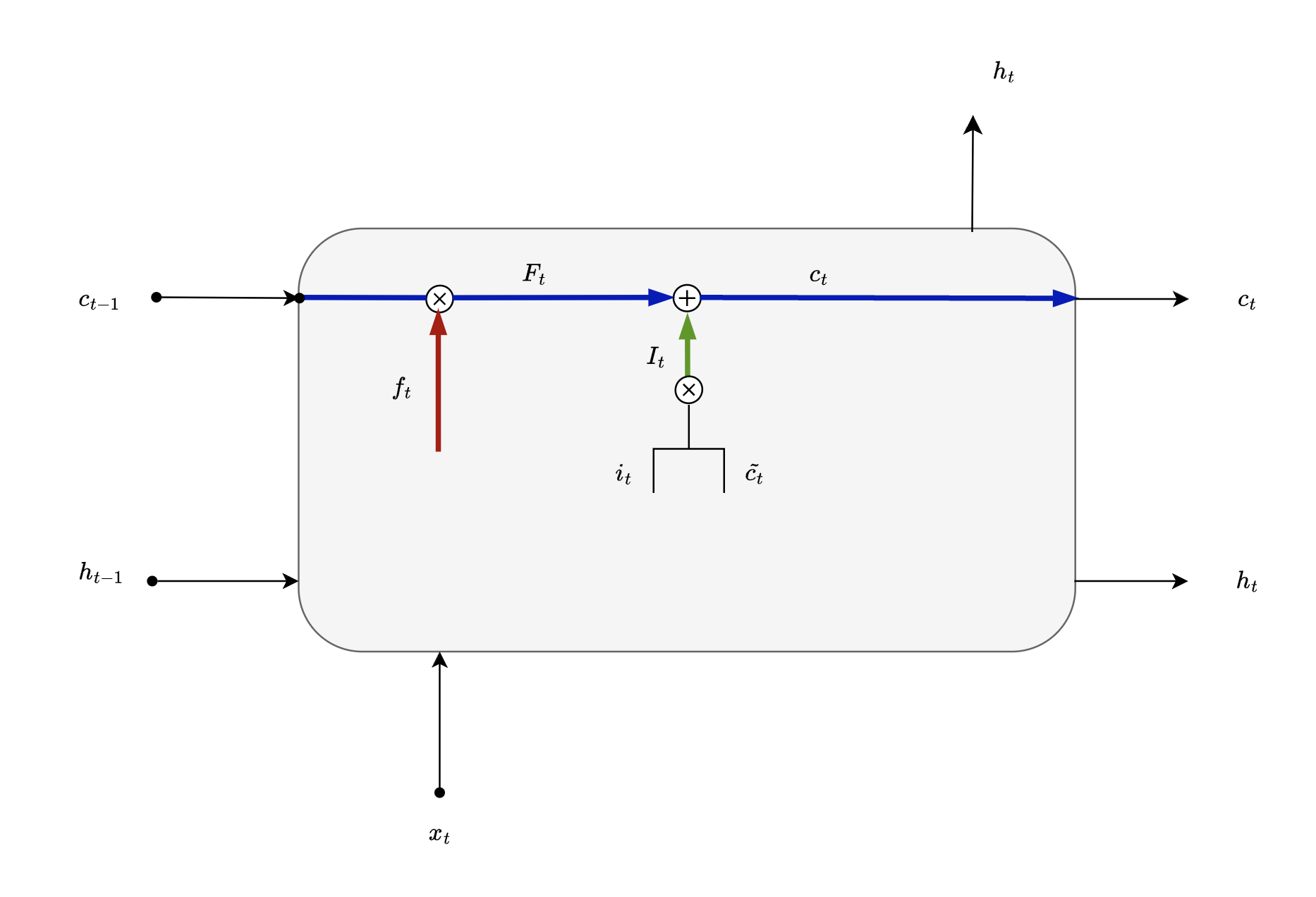
Notice how cell state at timestep is always a function of addition of two gated products, here forget gate and input gate .
Recall here
- how do we allow entire vector unchanged through the gate?
- vector of 1s -
[1,1,1,1,1]
- vector of 1s -
- how do we stop entire vector to pass through the gate?
- vector of 0s -
[0,0,0,0,0]
- vector of 0s -
Similar concept is applied here
How can we stop vectors at forget gate?
- when
- what happens to output of forget gate?
How can we stop vectors at input gate?
- when
- what happens to output of input gate?
Consider this simplified diagram where 3 time steps of LSTM are shown - let us view how information flows with respect to time step . The stickman figure at time step needs some information from previous time along the blue path shown below, let us see if LSTM is able to provide the same.
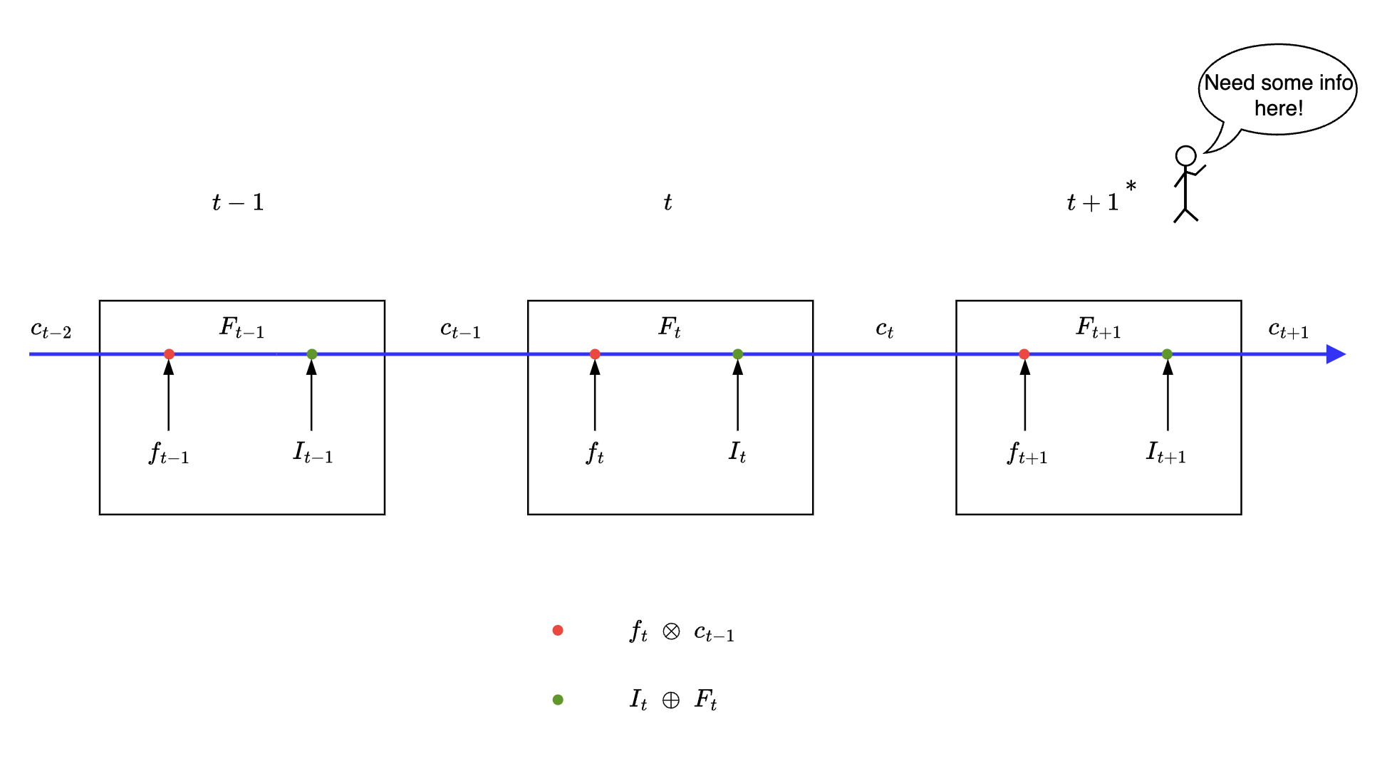
For ease of explanation
- means
- similarly for
where or
Case #1
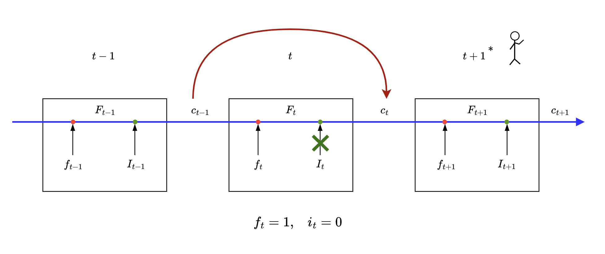

💬 i ONLY need NOT
This case is what enables LSTM to carry over long term memory.
Some math in action:
As we can see this type of gate setting in LSTM serves as a skip connection for cell state, skipping one or more states in between to reach to required time step.
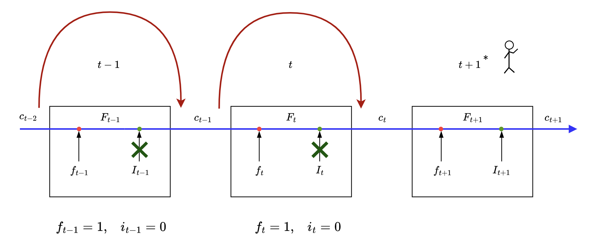
Imagine we need cell state from time step , all the intermediate gates between time step and will be set to where is index of intermediate time step.
Following diagram illustrates the same with
Case #2
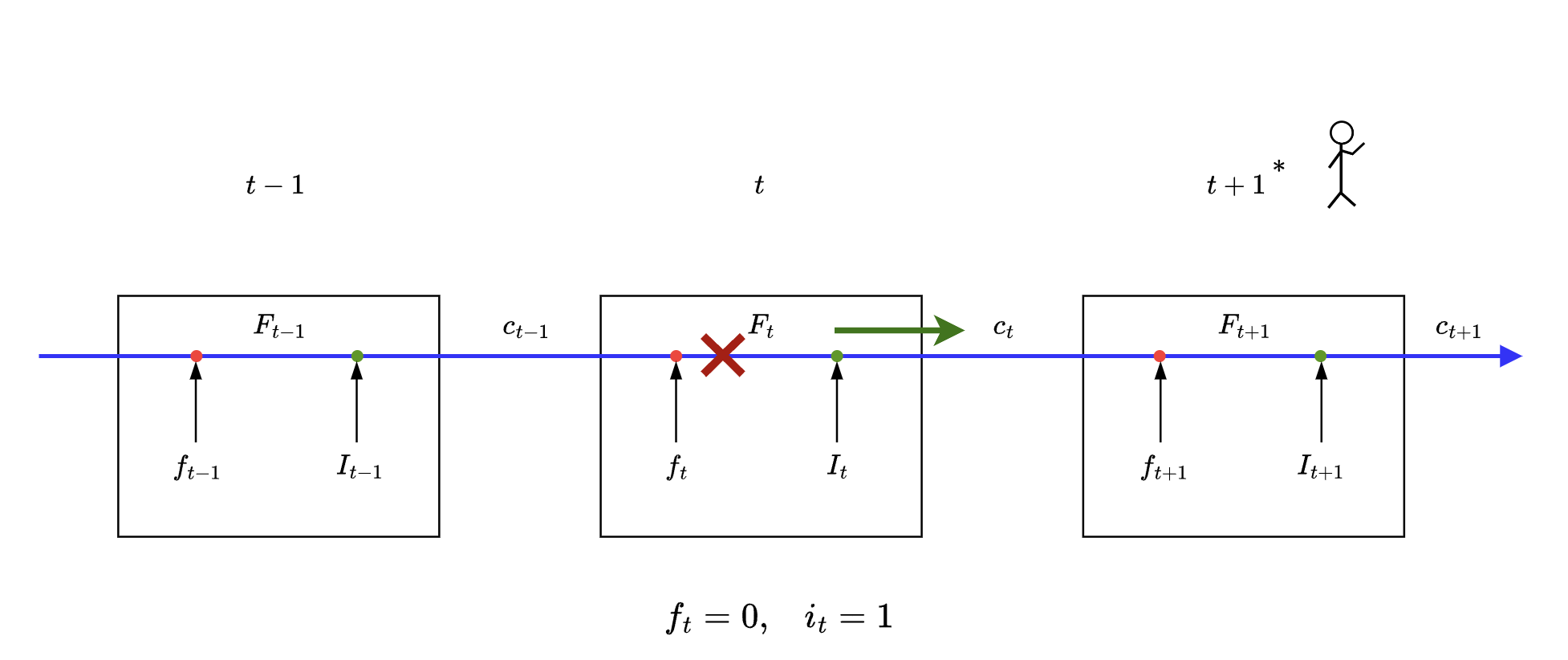
💬 i do NOT need cell states before time step
Again some math:
Here we can see that no vector passes through the forget gate and we use ONLY the output of input gate to generate cell state at time to be consumed at time step .
Case #3
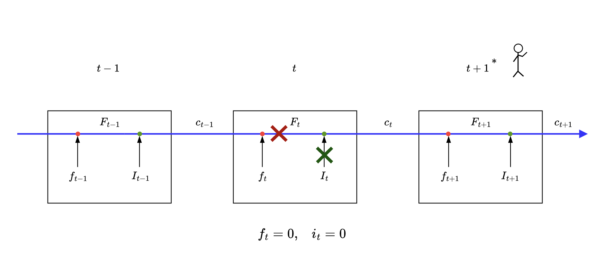
💬 i need a break
This is where LSTM
- erases all previous information
- and does NOT learn anything new
Mathematically
Here we can see that we allow both the vectors to pass through the forget gate and input gate respectively. Here we get information of both current state and states before it as some additive form of vectors mentioned above.
Case #4
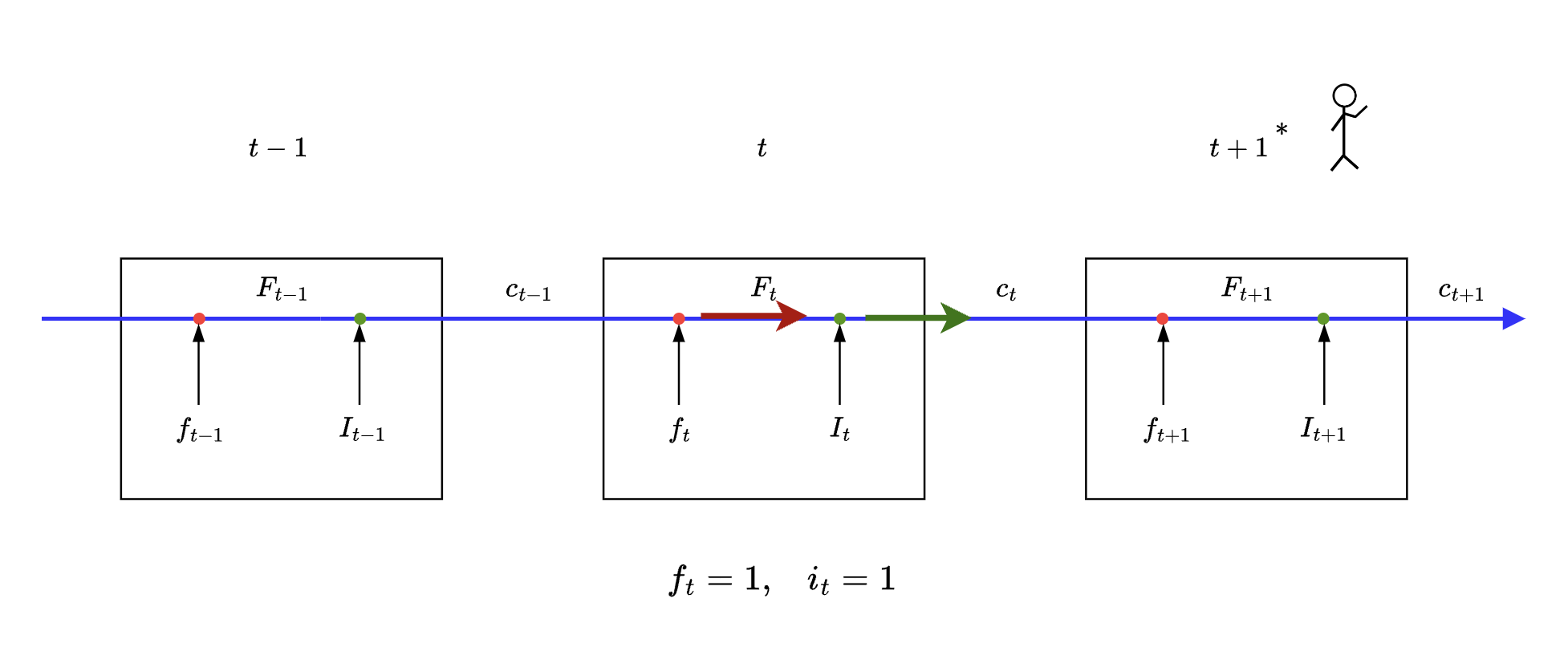
💬 i need gist of all the cell states in previous time steps
(can’t catch a break now can i?)
Mathematically
Here we can see that we allow both the vectors to pass through the forget gate and input gate respectively. Here we get information of both current state and states before it as some additive form of vectors mentioned above.
End note
This brings us to the end of this long blog. We covered how LSTMs use gated flow of vectors to retain both long and short term information, but there is still some ground left to cover, like how LSTM actually solve for vanishing gradient problem. This part is covered in detail in the references mentioned below. I hope reading this gave an in depth as well as intuitive understanding of LSTMs.
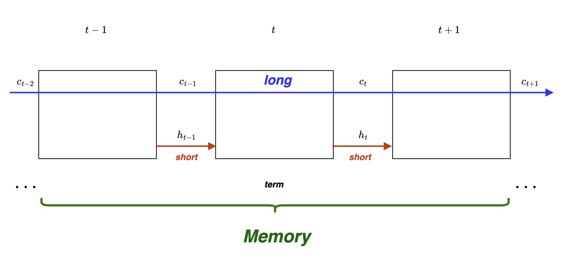
One final “diagrammatic” takeaway before ending this blog
This is how LSTMs keep a track of both long and short term memory
References
- This blog Understanding LSTM Networks by Christopher Olah is gold standard and helped me understand internal working of LSTMs. Huge shoutout. My blog is mere interpretation of the concepts explained here.
- CS Toronto slides
- Detailed walkthrough LSTMs (Video series)
- How LSTM networks solve the problem of vanishing gradients
- Back propagation using dependency graph
- How the LSTM improves the RNN