Precursors to Byte Latent Transformer
← back
Contents
- Introduction
- 50% lesser FLOPs
- Think Bytes, not Tokens
- Patching
- Types of Byte Patching
- Fixed K Byte Patching
- Space-based Patching
- Pros of Fixed K-size and Space-based Patching
- Cons of Fixed K-size and Space-based Patching
- Entropy based Patching
- What is Entropy mathematically?
- Why is Entropy important in patching?
- How does Entropy intuition translate into patching?
- Let's patch!
- Patching with a simple model
- But why Patch with entropy?
- End Note
- Appendix
- References

Introduction
Recently, Meta announced a tokenizer-free architecture called Byte Latent Transformer for language modelling. For the first time, this architecture matches tokenizer-based LLM performance at scale with a significant breakthrough: using up to 50% fewer FLOPs during inference.
50% lesser FLOPs
This is what got me into this rabbit hole!
| Users | Monthly Cost | Yearly Cost | GPUs Needed | What That Yearly Cost Could Buy |
|---|---|---|---|---|
| 1K | ~ $40K | ~ $500K | 8 A100s | A small apartment in most major cities worldwide |
| 100K | ~ $110K | ~ $1.3M | 16 A100s | A fleet of 20 luxury cars |
| 1M | ~ $460K | ~ $5.5M | 32 A100s | A mid-sized commercial building |
| 100M | ~ $30M | ~ $360M | 100+ A100s | A modern passenger aircraft |
Detailed calculations are available in the appendix.
These technical changes are no longer just about complexity reduction. They are about the pure economic scale at which AI is operating today. More efficient inference means more accessible AI, lower operational costs, and potentially faster response times.
This is Part 1 of a deep dive into Byte Latent Transformer where I will cover a few concepts that are required to get into the depths of this architecture and also provide a brief overview of this newly proposed architecture by Meta.
Before we dive deep, let's break down the key pieces required to learn this new architecture.
*tokenizer-free: for this blog refers to byte-based models which do not use tokenizers
Think Bytes, not Tokens
The fundamental difference between tokenizer-free architectures and token-based systems lies in their input processing and initialization.
Tokenizers need to be trained with multiple preprocessing steps on a large corpus to come up with a fixed set of vocabulary (~30K-50K items) for the model. To expand this vocabulary you need to re-train the tokenizer.

Whereas in the case of Byte-based systems, there is no concept of vocabulary as such. The real tricky part in tokenizer-free systems is how we make splits between the raw byte streams, more on that later.
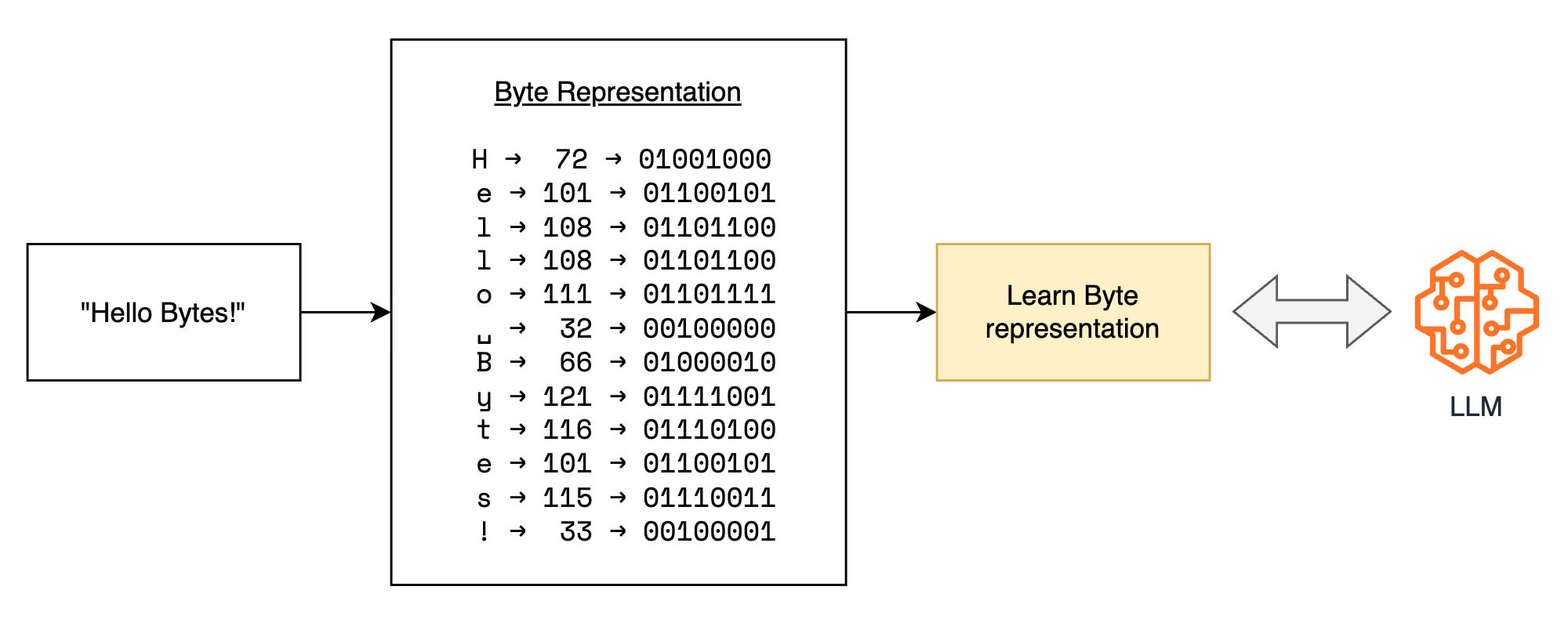
For now here are some major differences between these two systems:
| Aspect | Token-based Systems (Sentence piece, BPE) | Token-Free Systems (BLT, MegaByte, SpaceByte) |
|---|---|---|
| Training Data | Requires large corpus (>100GB) | No pre-training data needed |
| Vocabulary Size | 30,000-50,000 tokens | - |
| Vocabulary Growth | Grows with data/domains | Fixed size |
| Representation | Learned subword units | Raw UTF-8 bytes |
| Coverage | Limited by training corpus | Universal |
| Memory Usage | Higher (larger vocabulary) | Lower (smaller vocabulary) |
But how does using bytes instead of tokens make a difference?
Traditional tokenizer-based Large Language Models (LLMs) learn a unique embedding for each token in their vocabulary, which can be as large as 50,000 tokens. In contrast, by using byte representations, you only need to learn a very small set of byte representations. This significantly reduces the memory usage of the model.
Moreover, when expanding the domain knowledge or multilingual capabilities of a traditional LLM, the tokenizer requires additional training. This training process also increases the size of the model's embedding layer.
By encoding words or sentences into their fundamental byte representations, the need for a tokenizer is eliminated. This approach simplifies the process of extending the model's knowledge and multilingual capabilities without the overhead of tokenizer training and increased embedding layer size.
Is this all that there is to using Bytes instead of Tokens in BLT?
Multiple architectural changes have gone into this paper, which has resulted in significant results:
- BLT matches performance of Llama3 model while using 50% lesser FLOPs during inference
- BLT dynamically allocates compute to improve FLOP efficiency
- With BLT we can scale up model size while maintaining the same inference FLOP budget
- BLT is less prone to noisy inputs than token-based LLMs
Patching
But before we dive into technicalities, let’s talk about this diagram for a bit.

Training of tokenizers inherently teaches them the patterns of words and subwords, so we exactly know where the splits will occur when we use a tokenizer, whereas what if you are given a series of integers as an input?
- How will you decide on what the right partition (p1, p2, p3) is?
- What makes a partition the right one?
This art of splitting a long series of bytes into smaller groups/chunks is called patching and the formed groups are called patches in this paper, you use a patching function to get patches from byte stream.
Let us look into the type of patching where each one falls short and how BLT solve patching in the next few sections.
Types of Byte Patching
Fixed K Byte Patching
As the name suggests, after every K bytes we create a patch and move to create the next patch.

- We can see this leads to inconsistent and non-contextual patching of similar byte sequences - for example, the same word could be split differently in different contexts
- The fixed stride is simpler to implement and provides a straightforward mechanism for controlling FLOP cost, as patch size directly determines the compute required
- A key limitation is that compute is not dynamically allocated - the model uses the same transformer computation step whether processing informational bytes (like the start of a word) or more predictable content (like whitespace or punctuations)
Space-based Patching
Similarly here irrespective of the number of bytes each patch holds, you make a split where a space occurs.

- This type of patching gives more coherent patching as words stay together and are segmented consistently across sequences
- However, it has limited control over patch size and therefore compute costs, as patch lengths vary based on word lengths
- While it naturally allocates compute for harder predictions (like first bytes after spaces), it cannot gracefully handle all languages and domains
Below is a more comprehensive table, listing down strengths and limitations of fixed-size and space-based patching.
Pros of Fixed K-size and Space-based Patching
| Aspect | Fixed K-size Patching | Space-based Patching |
|---|---|---|
| Implementation | Simple fixed-size windows make implementation straightforward (e.g 16, 32, 64 bytes) | Simpler implementation than fixed size patching (e.g just split on the byte that represents <space>) |
| Control | Can easily switch between patch sizes (16->32->64) based on hardware constraints | Coherent splitting of bytes (e.g maintains meaningful byte sequences) |
| Performance | Predictable compute cost (e.g 1M tokens = exactly 62.5K patches of size 16) | Natural breaks in byte sequences guide the splitting |
Cons of Fixed K-size and Space-based Patching
| Aspect | Fixed K-size Patching | Space-based Patching |
|---|---|---|
| Resource Usage | Same resources for both simple and complex sequences | Cannot control patch size for optimization |
| Sequence Processing | Might split semantically related byte sequences incorrectly | Variable computational overhead between patches |
| Compatibility | Inconsistent handling of non-contiguous similar byte sequences | Not all languages and domains are handled effectively |
| Predictability | Semantic units split across patches affect prediction accuracy (e.g "this boo", "k was wr", “itten by”) | Prediction after certain sequences with punctuations might affect prediction accuracy (e.g "who wrote xyz book?<space>" → "?<space>") |
NOTE : there are other patching schemes/ functions like BPE, CNN based patching which are not discussed in this blog as they are slightly out of scope.
Entropy based Patching
What is Entropy mathematically?
Now that we have seen few types of patching, let's look into how BLT solves for patching. Instead of using rule based patching, BLT relies on a more data driven approach for patching.
Taken from the paper:
We train a small byte-level auto-regressive language model on the training data for BLT and compute next byte entropies under the LM distribution over the byte vocabulary :
This equation is called Claude Shannon's entropy equation. Let's break down this equation:
- is the entropy of the next byte
- is the probability of the next byte being given the previous bytes
- is the log probability of the next byte being given the previous bytes
Entropy is a measure of the uncertainty or randomness of a probability distribution. In this case, it measures the uncertainty of the next byte in the sequence given the previous bytes.
Why is Entropy important in patching?
Imagine you are talking to your friend on a call and you start the conversation with "Hello, how are you?" And your friend responds with one of the following:
- "Hello, I'm great!"
- "Flying Elephants in the zoo are very cute!"
Which of the above responses is more surprising? I think we all agree that the second response is more surprising, and extremely unlikely to be the response to the question "Hello, how are you?".
The entropy equation helps us measure how likely a byte sequence is. Just like we can tell if a sentence/word is highly unlikely, we can also measure how random a byte sequence is.
How does Entropy intuition translate into patching?
Researchers trained a small model to predict the entropy of the next byte given a byte sequence. So let's try to visualize and understand how this entropy model works with a diagram.
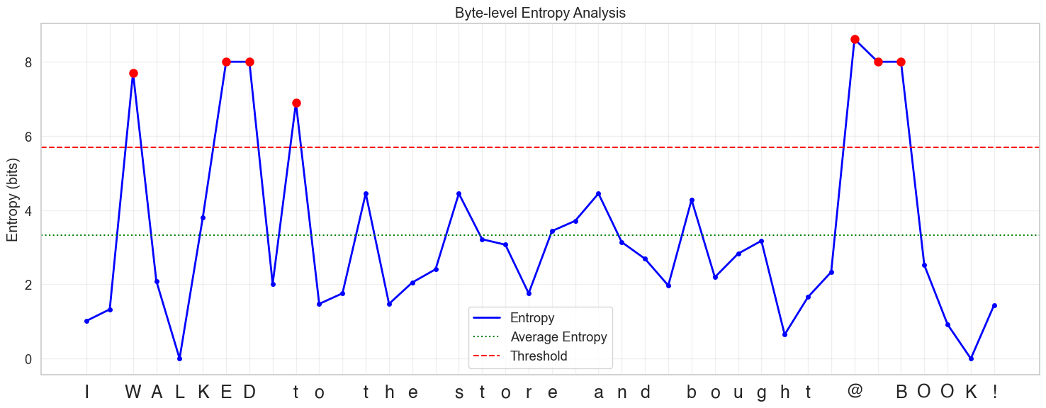
"I walked to the store and bought a book".
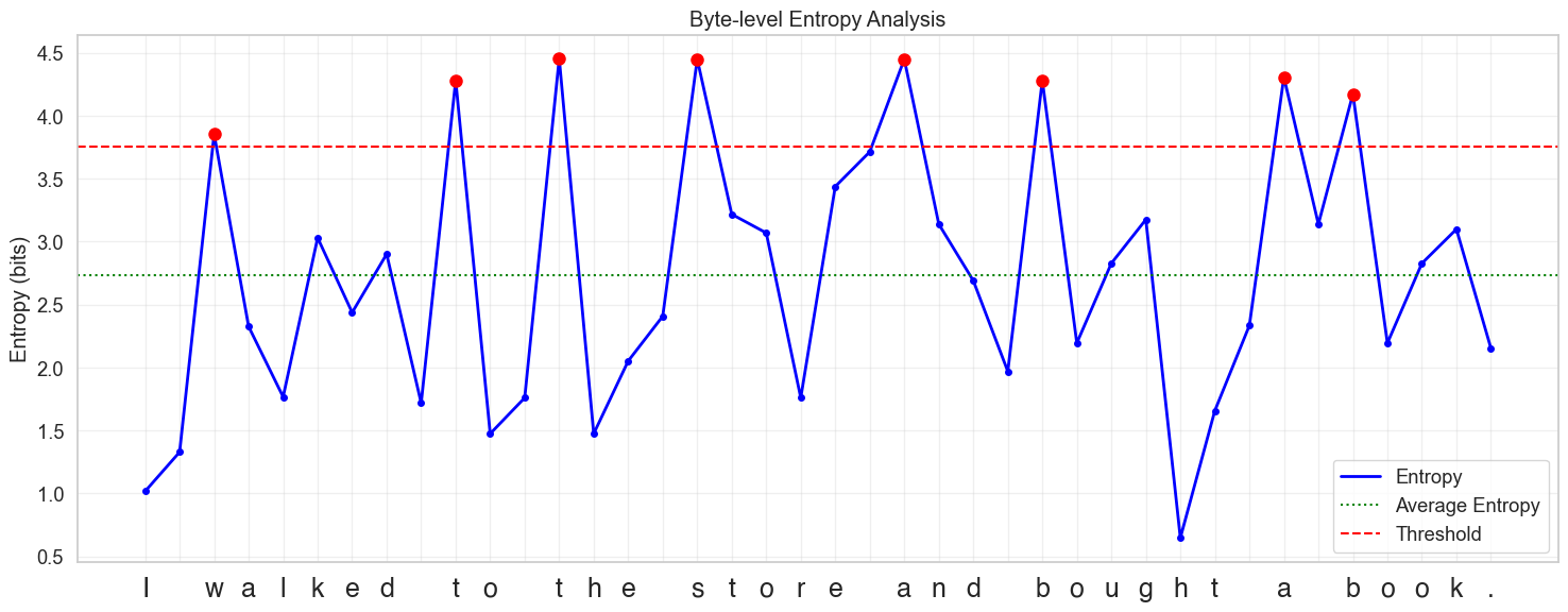
Key components of the diagram:
- Blue Line: Shows entropy values for each byte/character
- Red Dashed Line: Represents the entropy threshold
- Green Dotted Line: Shows the average entropy
- Red Dots: Marks high entropy points (peaks) where entropy exceeds the threshold
- Y-axis: Measures entropy is in bits
- X-axis: Individual bytes converted to characters in the sentence
Let's look more closely at this diagram now:
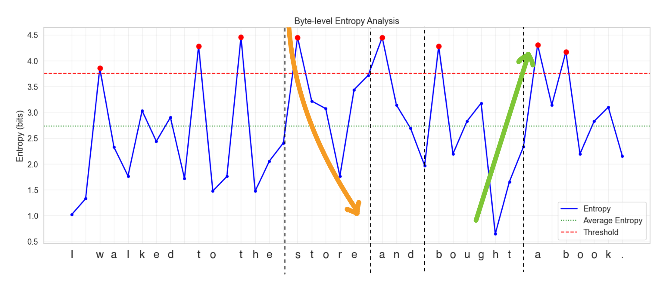
You can see that after every word there is a spike in entropy. And as you progress through a certain word, the entropy decreases gradually. A word can be bounded by dashed lines and can be considered as a patch.
Similarly, you can notice abnormalities in entropy values when you look at some unusual words and symbols in sentences, like "I WALKED to the store and bought @ BOOK!" in the diagram below.
Methods mentioned in the paper for patching
-
Global Constraint:
- Here you use a global threshold to determine a patch boundary
- In the above diagram you can see that the threshold is being set to some value in red dashed lines
- Every Red dot above the threshold marks the start/end of a patch
- Mathematically it can be represented as
-
Approximate Monotonic Constraint:
- Here you use a monotonic constraint to determine a patch boundary
- This constraint tries to answer if the entropy is consistently decreasing or not across the sequence
- Mathematically it can be represented as
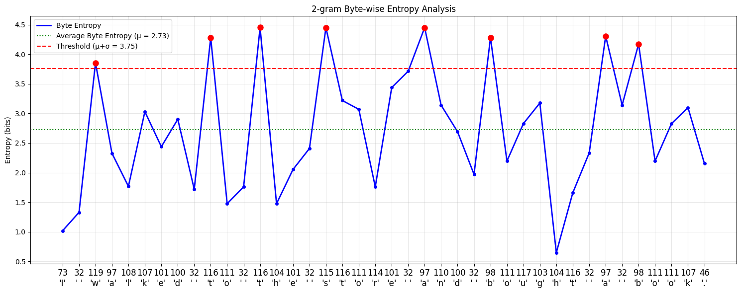
NOTE: All the diagrams below have different entropy values and thresholds, this is because the model is trained on a slightly larger dataset.
Let's patch!
Patching with a simple model
Let's try to see what patches are created using these methods seen in the previous section. I trained a small model (n-gram model with n=2) here to predict the entropy of the next byte given a byte sequence and plotted the patches created using the global constraint method and approximate monotonic constraint method.
Details
Patch 1: 'I ' (2 bytes)
Patch 2: 'w' (1 bytes)
Patch 3: 'alked ' (6 bytes)
Patch 4: 't' (1 bytes)
Patch 5: 'o ' (2 bytes)
Patch 6: 't' (1 bytes)
Patch 7: 'he ' (3 bytes)
Patch 8: 's' (1 bytes)
Patch 9: 'tore ' (5 bytes)
Patch 10: 'a' (1 bytes)
Patch 11: 'nd ' (3 bytes)
Patch 12: 'b' (1 bytes)
Patch 13: 'ought ' (6 bytes)
Patch 14: 'a' (1 bytes)
Patch 15: ' ' (1 bytes)
Patch 16: 'b' (1 bytes)
Patch 17: 'ook.' (4 bytes)
Details
Monotonic Constraint Patches:
Patch 1: 'I' (1 bytes)
Patch 2: ' ' (1 bytes)
Patch 3: 'wal' (3 bytes)
Patch 4: 'ke' (2 bytes)
Patch 5: 'd ' (2 bytes)
Patch 6: 'to' (2 bytes)
Patch 7: ' ' (1 bytes)
Patch 8: 'th' (2 bytes)
Patch 9: 'e' (1 bytes)
Patch 10: ' ' (1 bytes)
Patch 11: 'stor' (4 bytes)
Patch 12: 'e' (1 bytes)
Patch 13: ' ' (1 bytes)
Patch 14: 'and ' (4 bytes)
Patch 15: 'bo' (2 bytes)
Patch 16: 'u' (1 bytes)
Patch 17: 'gh' (2 bytes)
Patch 18: 't' (1 bytes)
Patch 19: ' ' (1 bytes)
Patch 20: 'a ' (2 bytes)
Patch 21: 'bo' (2 bytes)
Patch 22: 'o' (1 bytes)
Patch 23: 'k.' (2 bytes)
If you closely look at the outputs of both monotonic and global threshold patching, you can see that the patches created vary in size, but they are not coherent.
But why Patch with entropy?
So what did we even achieve here, with entropy-based patching?
While the previous outputs may not have provided complete clarity, here is another interesting result worth considering!
Input sentence: "Sherlock Holmes is a smart detective."
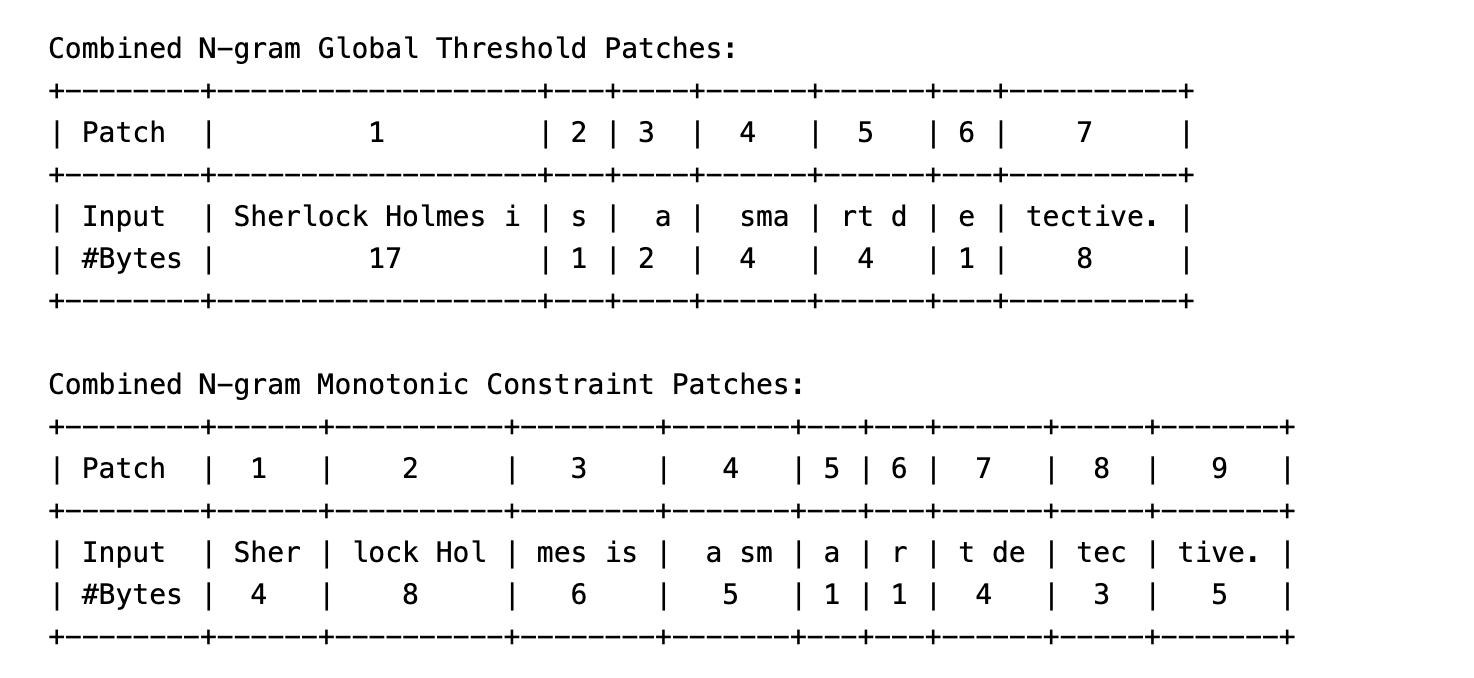
- Notice how the word
"Sherlock Holmes"is being combined into a single patch, this is because the entropy values are very low for the word"Sherlock Holmes"and the bytes forming this word frequently occur together in the corpus. - This is a good example of how entropy-based patching can create coherent patches, even for complex words.
The entropy values diagram for the above sentence are shown below.
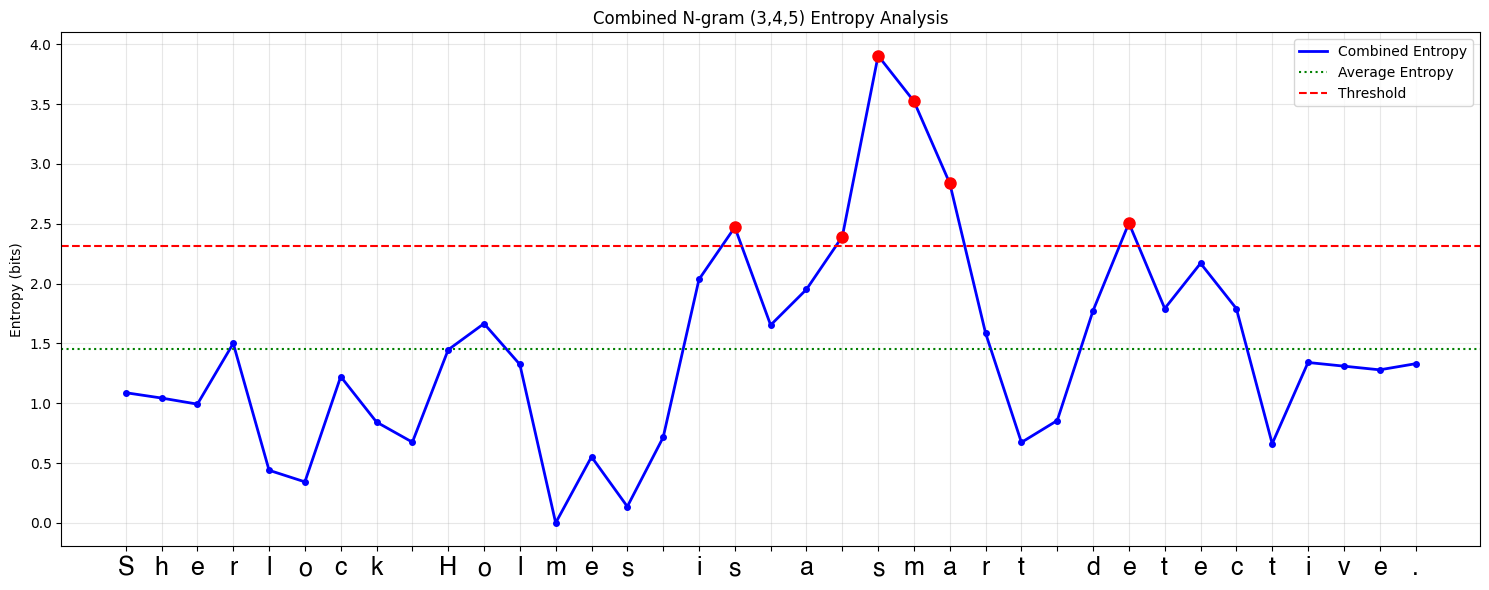
NOTE: This result was obtained using a better next-byte entropy prediction model using 3,4,5-gram models.
End Note
Additionally, this paper uses smart hacks to convert these dynamic patches to embeddings. It was important to establish the fact that patches of dynamic sizes can be created with entropy-based patching, and this can be achieved with simple models. The entropy-based patching model serves as an essential building block for BLT to achieve its performance.
Byte Latent Transformer architecture is shown below:
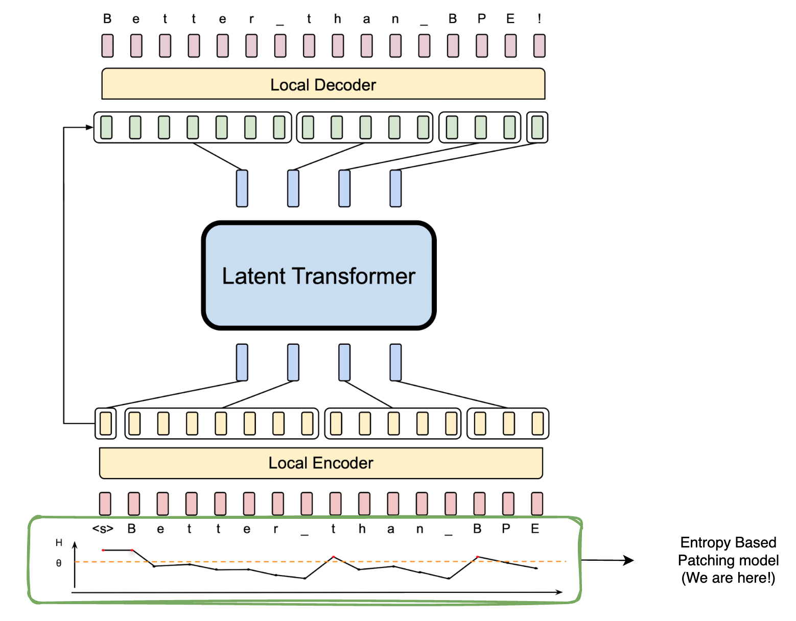
Well, we are just getting started, the next blog will cover how these patches are converted to embeddings how BLT, and how the inputs for the model are generated. It is going to be fun!
Appendix
-
Code for generating diagrams and artifacts in this blog is available on GitHub below:
- https://github.com/sagarsrc/exp-byte-latent-transformer
- I will be maintaining this repo for this blog and the upcoming ones.
- Feel free to experiment with the code and share your thoughts.
-
Details
Base Monthly Infrastructure Cost
$38/hour × 24 hours × 30 days = $27,360
With 1.5x redundancy: $27,360 × 1.5 = $41,040 base cost
Scaling factors for different user bases
1K users: 1x = $41,040
100K users: 2x = $82,080
1M users: 4x = $164,160
100M users: 12x = $492,480
Monthly inference cost per user
Tokens per request: 1,000
Requests per month: 10
Total tokens per user: 10,000
Cost per 1K tokens: $0.03
Monthly cost per user: (10,000 × $0.03) ÷ 1,000 = $0.30
Total monthly inference costs
1K users: $0.30 × 1,000 = $300
100K users: $0.30 × 100,000 = $30,000
1M users: $0.30 × 1,000,000 = $300,000
100M users: $0.30 × 100,000,000 = $30,000,000
Cost Summary Table
| Scale (Users) | Monthly Infrastructure Cost | Monthly Inference Cost | Total Monthly Cost | Annual Cost |
|---|---|---|---|---|
| 1K | $41,040 | $300 | $41,340 | $496,080 |
| 100K | $82,080 | $30,000 | $112,080 | $1,344,960 |
| 1M | $164,160 | $300,000 | $464,160 | $5,569,920 |
| 100M | $492,480 | $30,000,000 | $30,492,480 | $365,909,760 |
NOTE
These calculations are based on multiple assumptions:
-
User Behavior:
- Each user makes about 10 queries per month
- Average query is like a paragraph of text back and forth
- Usage is spread throughout the month (no major spikes)
-
Cost Components:
- Server costs: ~30K/month for base setup (8 A100s)
- Processing costs: ~30¢ per user per month