Introduction#

Positional encoding is a small concept in Transformer architecture yet of crucial importance. In RNNs or LSTMs we pass tokens sequentially, here information of "order" is inherently captured.

Whereas in the case of Transformers, we pass multiple tokens at the same time, they are more likely to lose out on positional information of tokens. As we are feeding tokens parallel we need to use some mechanism to remember the "order" of the tokens being fed to the transformer. Hence Positional Encoding.

Why position matters?

"the cat was chasing the mouse in the house"
"the mouse was chasing the cat in the house"

As we can see by swapping 2 words in the sentence, the whole meaning changes.

Goal#

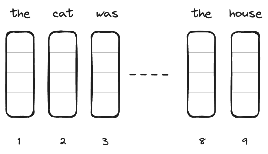
Model uses these words as embeddings, our goal is to make these embeddings carry additional position information, here the corresponding index associated with each word.

Proposed method#

Authors of "Attention Is All You Need" propose a novel method for encoding positional information. Below is the formulation.

$PE\_{(pos,2i)} = sin({pos}/{{10000}^{{2i}/{d}}})$

$PE\_{(pos,2i+1)} = cos({pos}/{{10000}^{{2i}/{d}}})$

Understanding variables:

variable	meaning
$w_0, w_1, .. w_n$	Words/ tokens in sequence
$i$	Index of embedding dimension
$pos$	position of word in sequence
$d$	embedding dimension of model

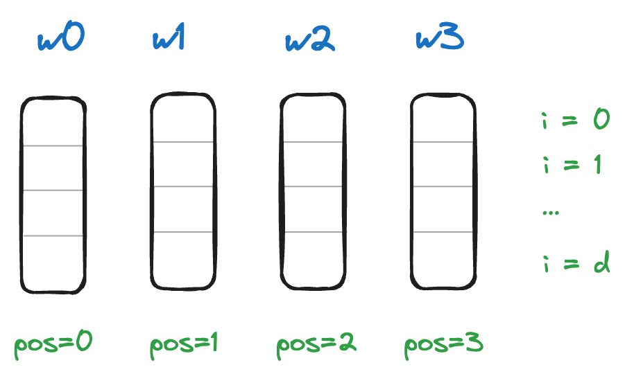
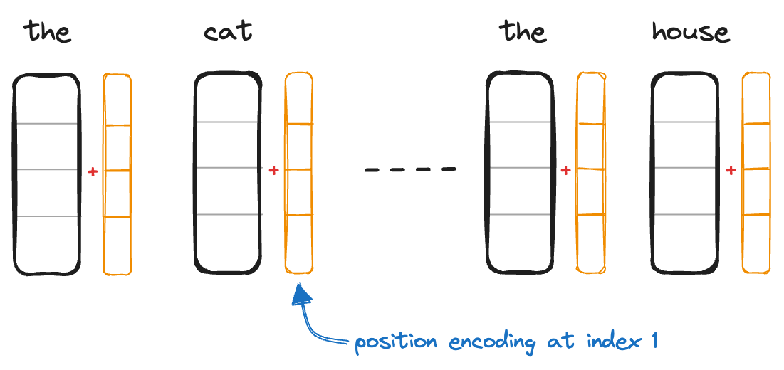
$fig\ 1$

This position embedding is further added with the word embedding as shown above. Let us try to understand what extra information the "orange" vector adds to word embeddings.

Breaking down Math#

For this blog let's choose embedding dimension size $d=512$

step 1 - formulation#

As we can see here two operations are being performed on an even index of embedding dimension for a given position. All even indices are some function of sine and odd indices are some function of cosine.

$PE\_{(pos,2i)} = sin(\theta)$

$PE\_{(pos,2i+1)} = cos(\theta)$

Where $\theta$ is a function of $pos$ and $i$

$\theta = {pos}/{{10000}^{{2i}/{d}}}$ $\theta = {pos} \* {1}/{{10000}^{{2i}/{d}}}$

$pos$ is just a multiplying factor
whereas division term ${1}/{{10000}^{{2i}/{d}}}$

step 2 - division term#

Let us try to plot this division term. ${1}/{{10000}^{{2i}/{d}}}$

$fig\ 2$

As we can see ${1}/{{10000}^{{2i}/{d}}}$ is a decaying function which ranges between $(0,1]$

step 3 - offset#

On multiplying $pos$ term with division term. $\theta = {pos} \* {1}/{{10000}^{{2i}/{d}}}$

$fig\ 3$

Multiplying $pos$ works as an offset for each position. Notice how each word's 0th dimension starts from a different point on the +ve y-axis and diminishes as we move towards the +ve x-axis

step 4 - even/odd $i$ #

Now for each even index applying sine function, and for each odd index applying cosine function.

$PE\_{(pos,2i)} = sin(\theta)$

$PE\_{(pos,2i+1)} = cos(\theta)$

$fig\ 4$

One interesting thing to note here is how all even indices at every position converge to 0
Similarly, all the odd indices at every position converge to 1 as we go deeper in the dimension (as $i$ increases)

Now let us put all these steps together and see how position embedding varies when we combine both even and odd index values

step 5 - oscillation#

This Plot tells us how the value of position encoding varies across dimension $i$ for each word at position $pos$ . We can see that each encoding varies as we go to a different position. Values for any position $pos=p$ will remain the same irrespective of number of words in the sentence.

$fig\ 5.1$

We can further visualize the same positional encoding for say 100 words as a heatmap to see overall variation in the values of these vectors.

$fig\ 5.2$

One can observe similar patterns in both $fig\ 5.1$ and $fig\ 5.2$ :

There is a higher variation in the range of [-1, 1] seen in the initial dimensions of a positional vector
Whereas as we go towards later dimensions of the positional vector this oscillation ranges between [0, 1]

Usage#

Let's revisit the older diagram we began with. In the above steps, we saw how each position $pos$ can be represented uniquely. Now we have the "orange" vector which has positional information in it.

We add each word embedding at $pos=n$ with corresponding position encoding.

$\vec{w_{n}} = \vec{e_{n}} + \vec{p_{n}}$

Each vector $\vec{w_{n}}$ , where $n\ \epsilon\ [0,1, ... N]$ is given as an input to transformer.

symbol	meaning
$N$	total number of words
$\vec{w_{n}}$	word embedding with positional information at $pos = n$
$\vec{e_{n}}$	word embedding of word at $pos = n$
$\vec{p_{n}}$	position encoding for word at $pos = n$

Code implementation#

import numpy as np
 
def positional_encoding(max_len, d):
    """
    Generate positional encodings for sequences.
 
    Args:
        max_len (int): Maximum length of the sequence.
        d (int): Dimensionality of the positional encodings.
 
    Returns:
        numpy.ndarray: Positional encodings matrix of shape (max_len, d).
    """
    position = np.expand_dims(np.arange(0, max_len, dtype=np.float32), axis=-1)
 
    # div_term is common for odd and even indices
    # operation done on these indices varies
    # hence size of `div_term` will be half that of `d`
    div_term = np.exp(np.arange(0, d, 2) * (-np.log(10000.0) / d))
 
    # placeholder for position encoding
    pe = np.zeros((max_len, d))
 
    # fill all even indices with sin(θ)
    pe[:, 0::2] = np.sin(position * div_term)
 
    # fill all odd indices with cos(θ)
    pe[:, 1::2] = np.cos(position * div_term)
 
    return pe, div_term
 
# call
max_len = 100
d = 512
 
positional_encodings, div_term = positional_encoding(max_len, d)
print("div_term shape:", div_term.shape)
print("Positional encodings shape:", positional_encodings.shape)

Summary#

This blog provides a visual mathematical guide to how a small component "position encoding" in transformer architecture works. I hope this gave you a fresh and in-depth perspective on the topic.

Reference#

Written by Sagar Sarkale

Position Encoding in Transformers