Introduction
Transformer architecture in the paper Attention Is All You Need might seem intimidating at first, given the number of prerequisites one needs to know before taking a shot at reading the paper or any blog around this topic. Here i try and attempt my version of breaking down the transformer architecture. While giving enough intuitive understanding of why certain things exist in the architecture, i also try to explain the transformations of matrices along the pipeline.
Also, this post is an inspired one many thanks to Andrej Karpathy and his recent work and all the other fellow researchers who went way beyond to explain this mammoth concept.
At first, there will be too many moving pieces, make sure you spend some time with the diagrams mentioned in each section to understand the flow in each step.
Structure
By now you might have seen the image below multiple times.
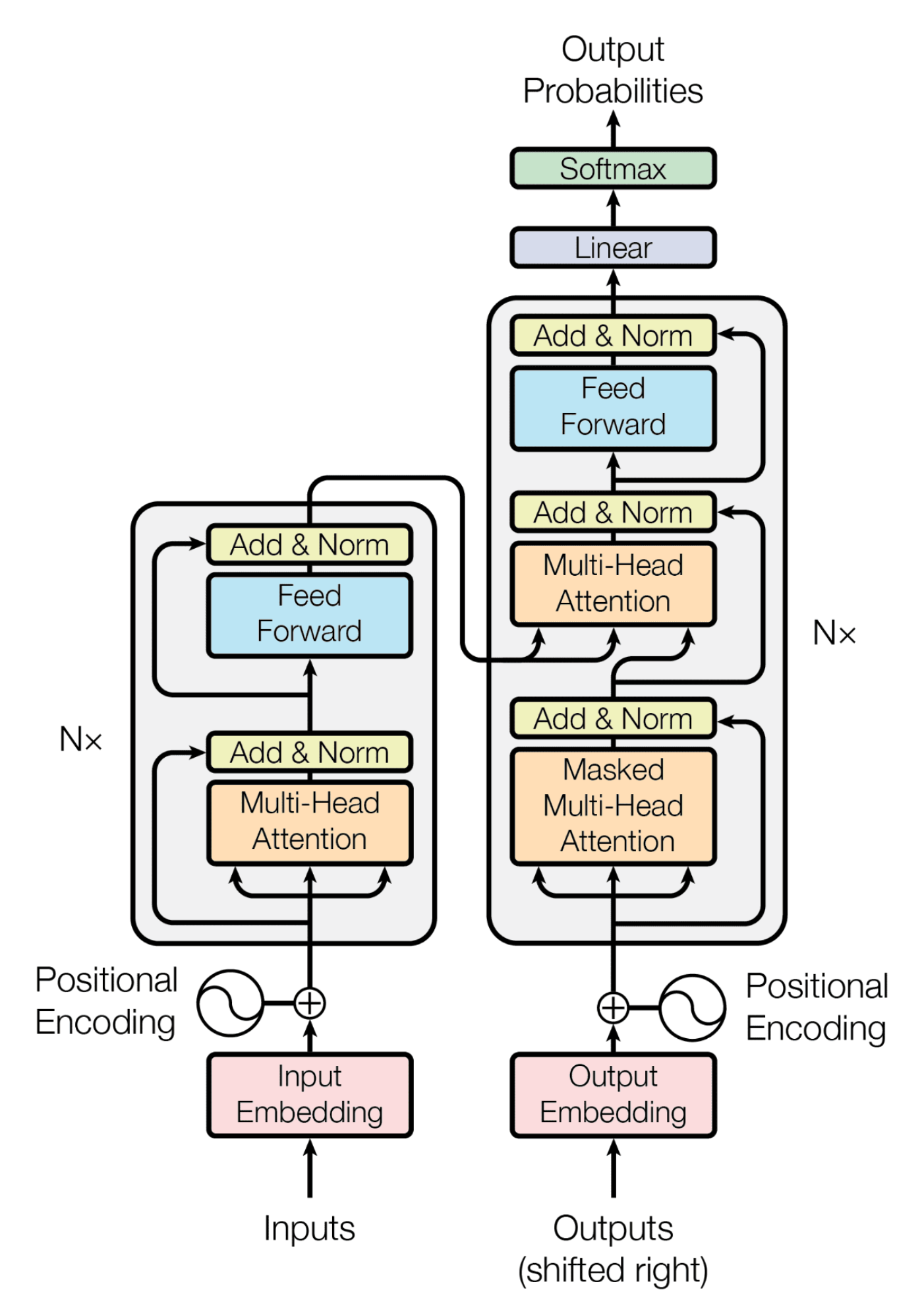
At its core, the Transformer consists of two main components: the encoder (represented by the grey block on the left) and the decoder (the grey block on the right).
In the years following the Transformer’s debut (2017), we’ve witnessed an series of innovative architectures. BERT (2018) released by Google, showcased the power of encoder-only models for understanding context in language. Meanwhile, OpenAI’s GPT, Meta’s Llama, series demonstrated capabilities of decoder-only models in generating human-like text.
Let us deep dive into decoder only architecture. Why?
- Decoder-only models like GPT-3, GPT-4, and LLaMA are at the forefront of AI research and applications.
- The architecture of decoder-only models is relatively straightforward, making them easier to explain and understand.
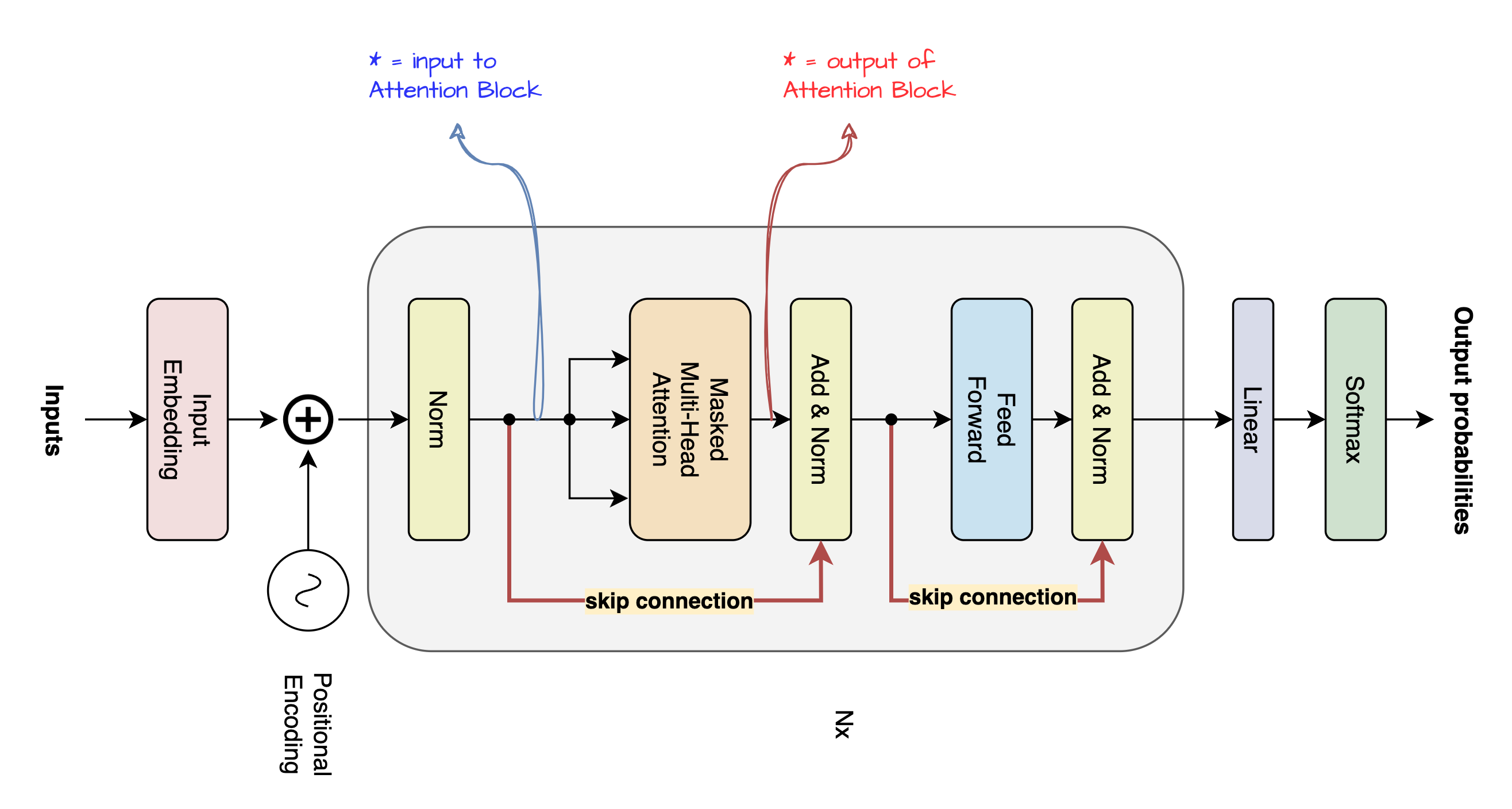
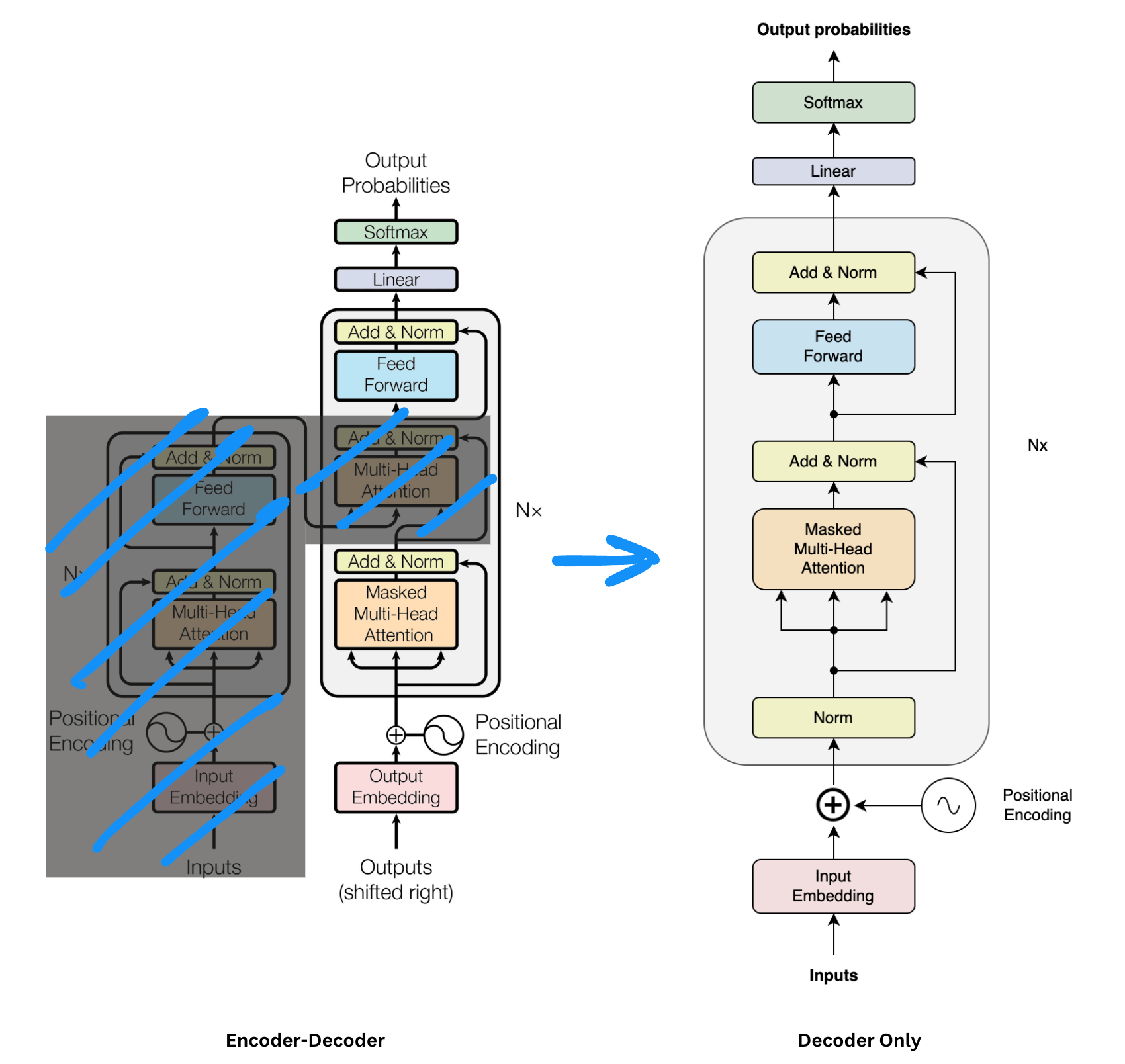
After removing encoder from the picture our architecture looks something like the image below. Let us try to break down how this kind of model works step by step.
Notations
| symbol | meaning |
|---|---|
| T | number of tokens |
| vocab_size | vocabulary size |
| ndim | dimensions of embedding |
For this blog let us choose
- number of tokens T = 6
- ndim = 768
Through all the steps below batch_size = 1 for simplicity. Additionally, each matrix has a footer like section denoting shape of the matrix.
Step 1 - Representing a sequence
Inputs (Step 1)
This is where any input sentence is converted to respective tokens using tokenizer and further converted to embeddings. Additionally we add a vector to each of the represented token to encode sequential information, there are multiple ways to get this vector for now we are skipping that.
For more information how we get position encoding and why we use position encoding read my previous blog here.
Outputs (Step 1)
Vectors representing tokens of input sequence and respective positions.
Step 2 - QKV matrices and splits
Inputs (Step 2)
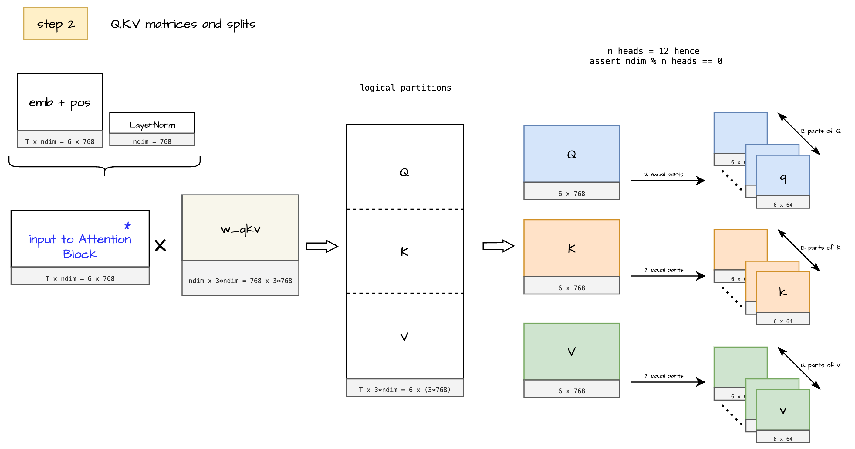
In this step we prepare inputs for calculating attention. We use existing token emebddings with positional information, and do Layer Normalization.
Brief on Layer Normalization:
[6 x 768]- Input $I$[6 x 1]- mean $\mu$ across feature dimension here 768[6 x 1]- variance $\sigma^2$ across feature dimension here 768[6 x 768]- Output = $({I - \mu})/{\sigma^2}$
The obtained result is further passed for matrix multiplication which give us matrices Query, Key, Value which is the crucial for calculating attention.
The model uses a single shared weight matrix, which is logically divided into separate parts for Q, K, and V. These divisions are shown as distinct matrices merely for easier visualization and understanding. Notice, the shape of w_qkv is [ndim x 3*ndim] , which on multiplying with input matrix [T x ndim] gives a [T x 3*ndim] shape resultant matrix.
Outputs (Step 2)
Notice how Q, K, V matrices are further broken down into smaller q, k, v matrices this is the output of step 2.
Let us remember this output of step 2. Each of the Q, K, V matrix is broken down into subgroups as follows:
- Q
[6 x 768]→[12 x 6 x 64]→[q1, q2, … q12] - K
[6 x 768]→[12 x 6 x 64]→[k1, k2, … k12] - V
[6 x 768]→[12 x 6 x 64]→[v1, v2, … v12]
Each of QKV matrices are split further into qkv matrices
12 groups each of shape
[6 x 64]
Step 3 - Self-attention mechanism
Everytime you google Attention you see this closed form of attention and mentions of query, key, value:
$\text{Attention}(Q, K, V) = \text{softmax}\left(\frac{QK^T}{\sqrt{d_k}}\right) V$
But what are - Q, K, V matrices?
Why do these matrices exist?
Let us try to understand this visually with a dummy sentence.
S : "Curious kid picked the apple”
By looking at sentence S we know that - kid has a certain quality (curious), and he has done some action (picking up the apple)?
How did we identify that? - Given a word “kid” we got corresponding relevant words in the sentence which are - “curious”, “picked”, “apple”.
Now observe the heatmap below, it is a representation of how Query and Key matrices are collectively used to capture these relevance scores.
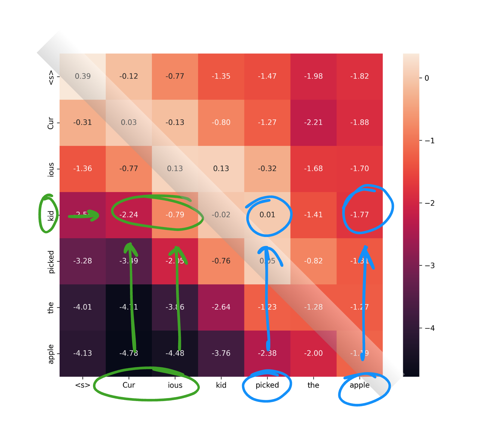
On the Y axis of this heatmap we have Queries, and on the X axis we have Keys, as you might have noticed there is some score associated between the words of sentence itself. Now you know why the term “Self” in “Self-Attention”. But wait we are not there yet “Attention” is not far away.
Notice how from this heat map we are able to find out keywords relevant to “kid”:
- “curious” - marked with green marker
- “picked”, “apple” - marked in blue marker
Some comments:
- For now let us have this convention all the corresponding scores for a key beyond the diagonal are marked in blue. Why? We will get to it soon.
- Also notice how values on the diagnoal are closer to 0, and comparison of key == value is leading to high relevance score
On multiplying Query and Key matrix we have pairwise relevance score, but these scores need to be converted into word representation with “modified relevance”. That is where Value matrix comes into picture.

So, essentially Value matrix is a projection to bring relevance scores to word representation with additional information of relevance. Above diagram only shows the overall transformation of matrix, there are additional operations that happen while calculating attention
Let’s go through that now.
The equation should look less daunting now. I hope that is the case!
$\text{Attention}(Q, K, V) = \text{softmax}\left(\frac{QK^T}{\sqrt{d_k}}\right) V$
Let’s break down this equation anyways.
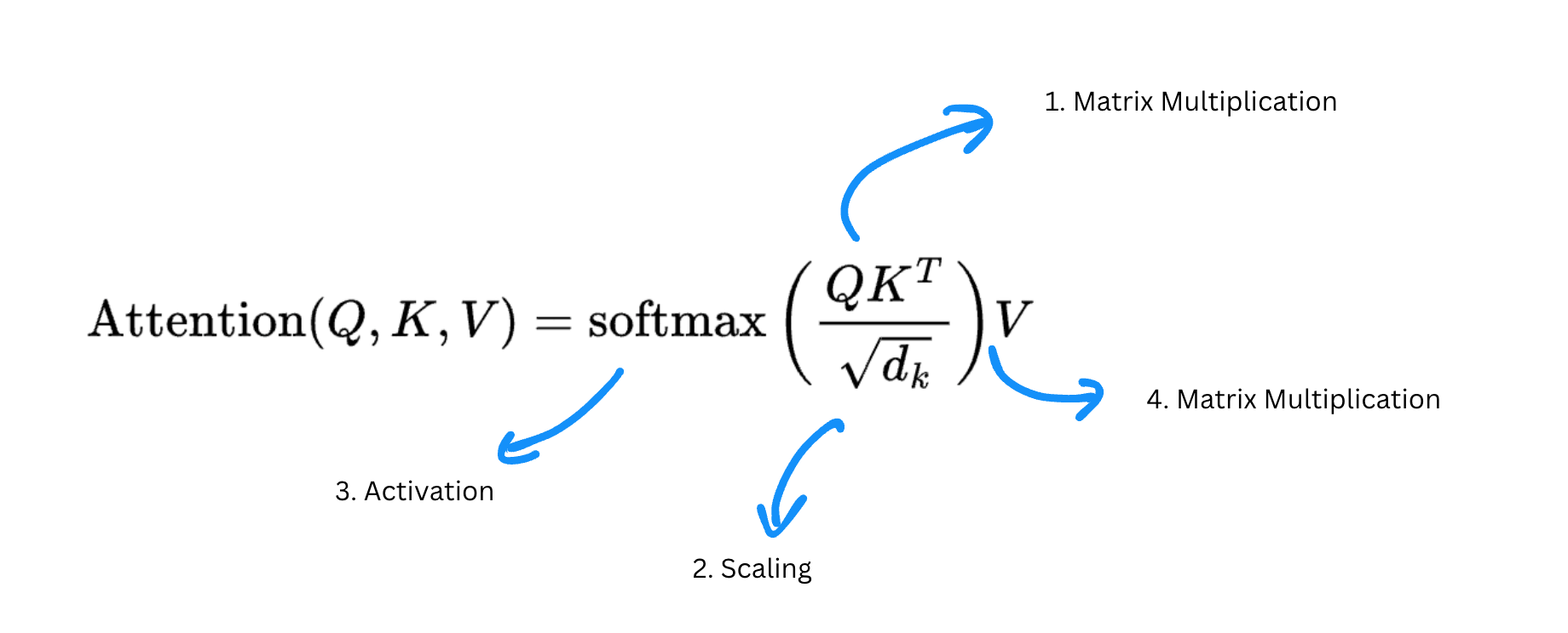
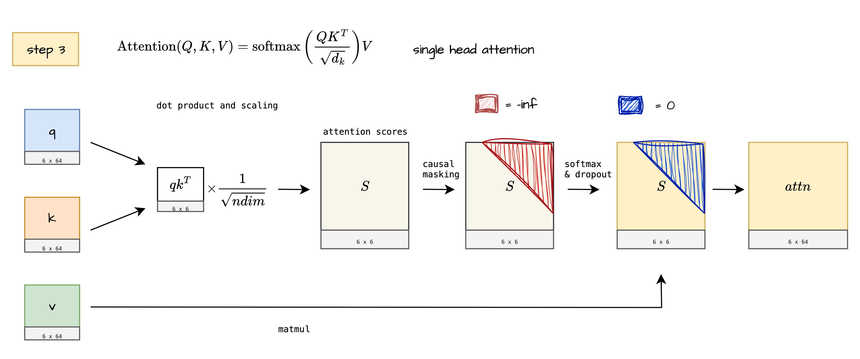
Let us see a block diagram for the same and understand how the shapes of matrices change.
Inputs (Step 3)
- Q
[6 x 768]→[12 x 6 x 64]→[q1, q2, … q12] - K
[6 x 768]→[12 x 6 x 64]→[k1, k2, … k12] - V
[6 x 768]→[12 x 6 x 64]→[v1, v2, … v12]
Each of the above QKV matrices can be though of as 12 groups of [6 x 64] matrices.
Let’s do operations on q, k, v each of shape [6 x 64].
- Multiply $q$ and $k^T$
- Scale it by multiplying with : ${1}/{\sqrt{ndim}}$
- Get relevance scores - also called as “attention scores”
- Apply causal masking step
- Get single head “raw attention output”
(On repeating the same process for 12 parts of Q, K, V we get multi-head attention)
By now we have some overall understanding about the overall flow of attention using q, k, v matrices. Let us touch on some of the steps that were skipped in the above section.
Scaling
On multiplying $q$ and $k^T$ we might get extremely large values in order to avoid that we scale the product down by multiplying it by $\frac{1}{\sqrt{ndim}}$.
Causal Mask and softmax
Well this is a neat trick to not allow our model to cheat while doing causal language modelling. As most of the language models predict next token given a bunch of tokens, masking attention scores tokens in future allow us to not attend to tokens that our model has not seen yet.
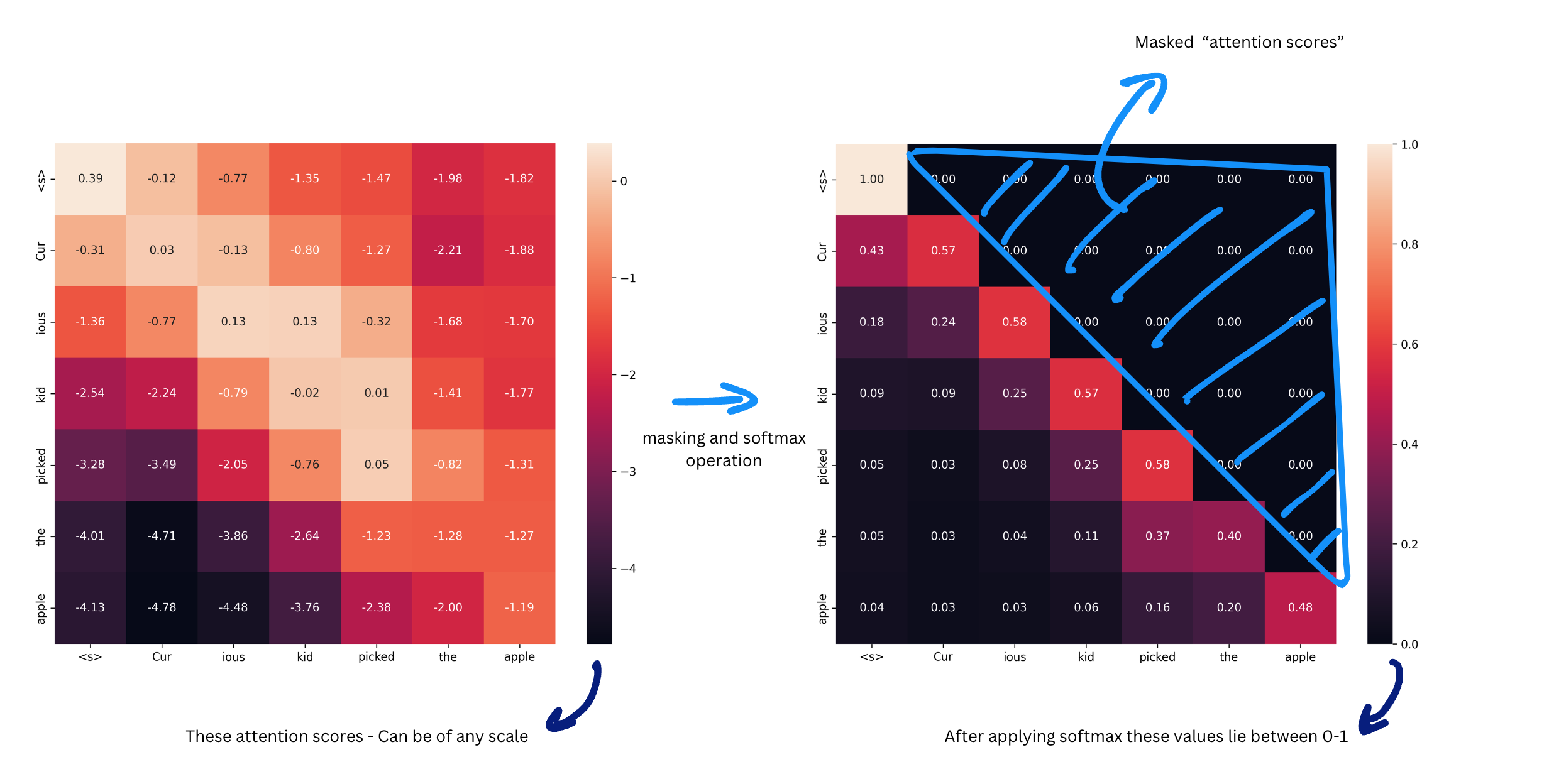
Objective while training is given tokens ["Cur", "ious", "kid"] predict ["picked"]. By masking attention scores we avoid model to learn from the attention scores of the tokens that are yet to be seen by model.
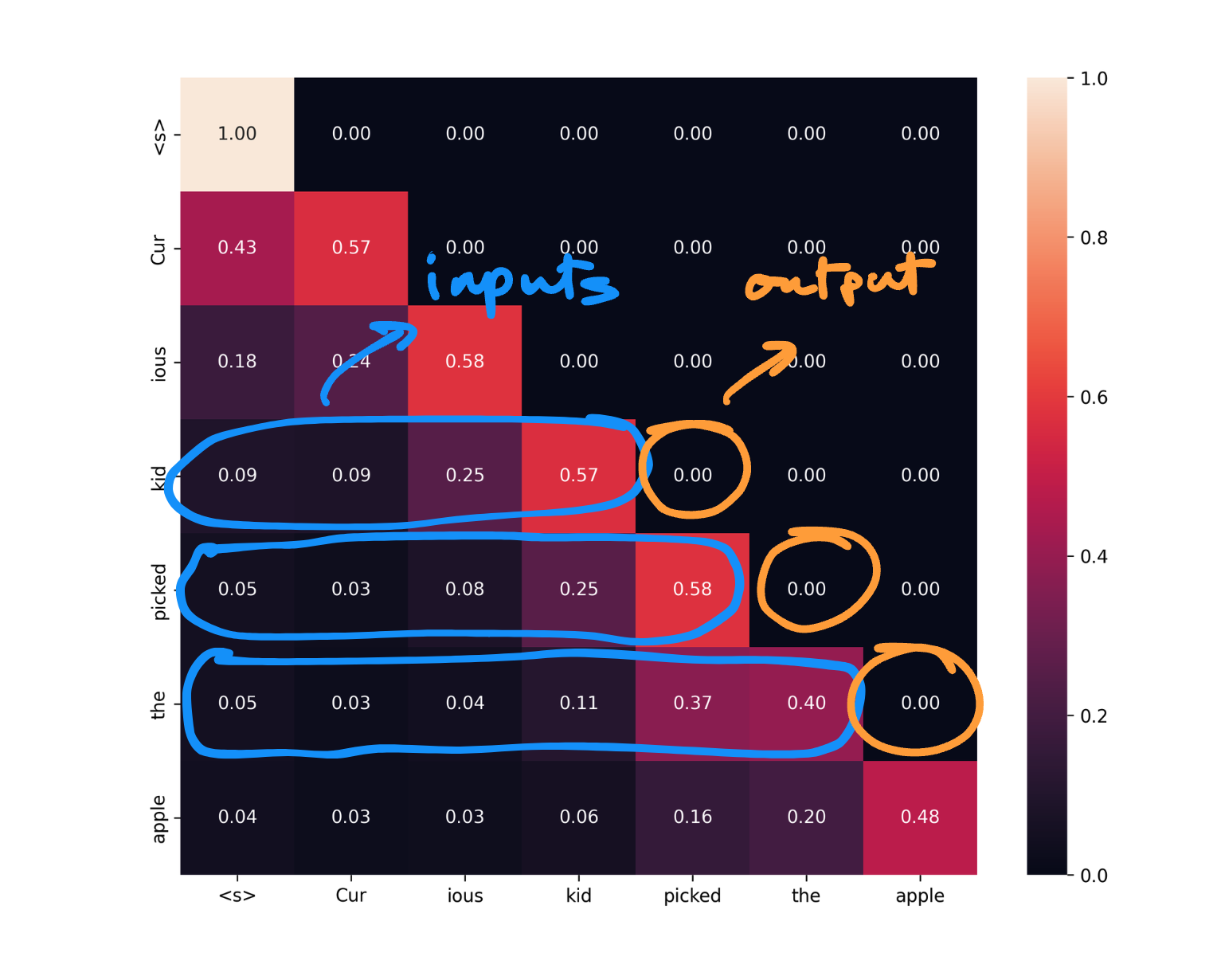
Same applies for other rows in the matrix, given tokens ["Cur", "ious", "kid", "picked"] predict ["the"] , and so on. One thing to note here is unline RNN or LSTM, calculation of losses can happen parallely (without having to wait for each timestep).
Now that we have all the moving pieces in attention we are ready to multiply values matrix with attention scores.
Values matrix
As mentioned above
On multiplying Query and Key matrix we have pairwise relevance score, but these scores need to be converted into word representation with “modified relevance”. That is where Value matrix comes into picture.
| Name | Dimensions | Description |
|---|---|---|
| S | [6 x 6] | Causal masked attention scores |
| v | [6 x 64] | Part of values matrix |
| A | [6 x 64] | Raw attention output result of Matrix multiplication of S and v |
Word “raw” is used as there are still some final transformations that these matrix goes through to get final attention output of the attention block.
This marks the output of Step 3 and is called as Single head attention.
Outputs (Step 3)
A [6 x 64] - single head raw attention output.
Step 4 - Multi-head attention
Inputs (Step 4)
Inputs are same as inputs in Step 3
Process
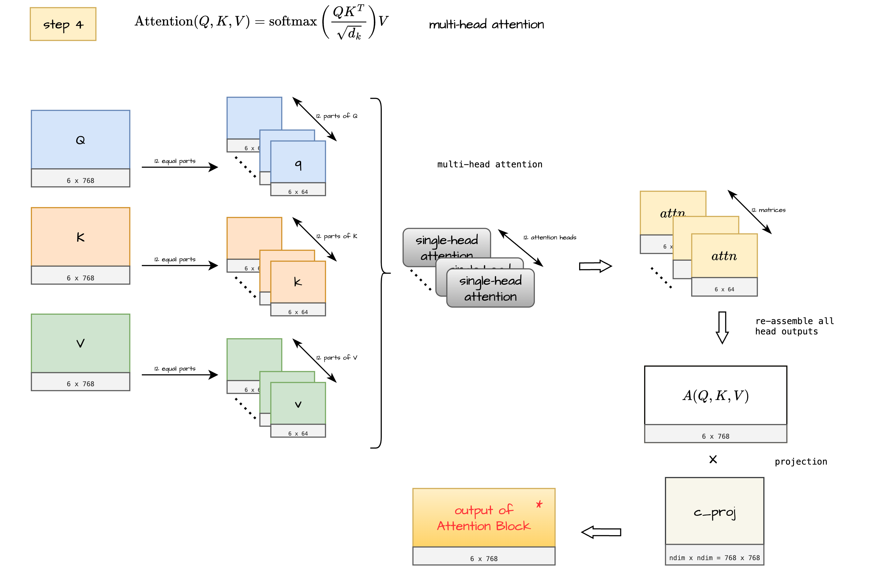
In this step we stack all the $attn$ matrices i.e all “raw attention outputs” into one large matrix.
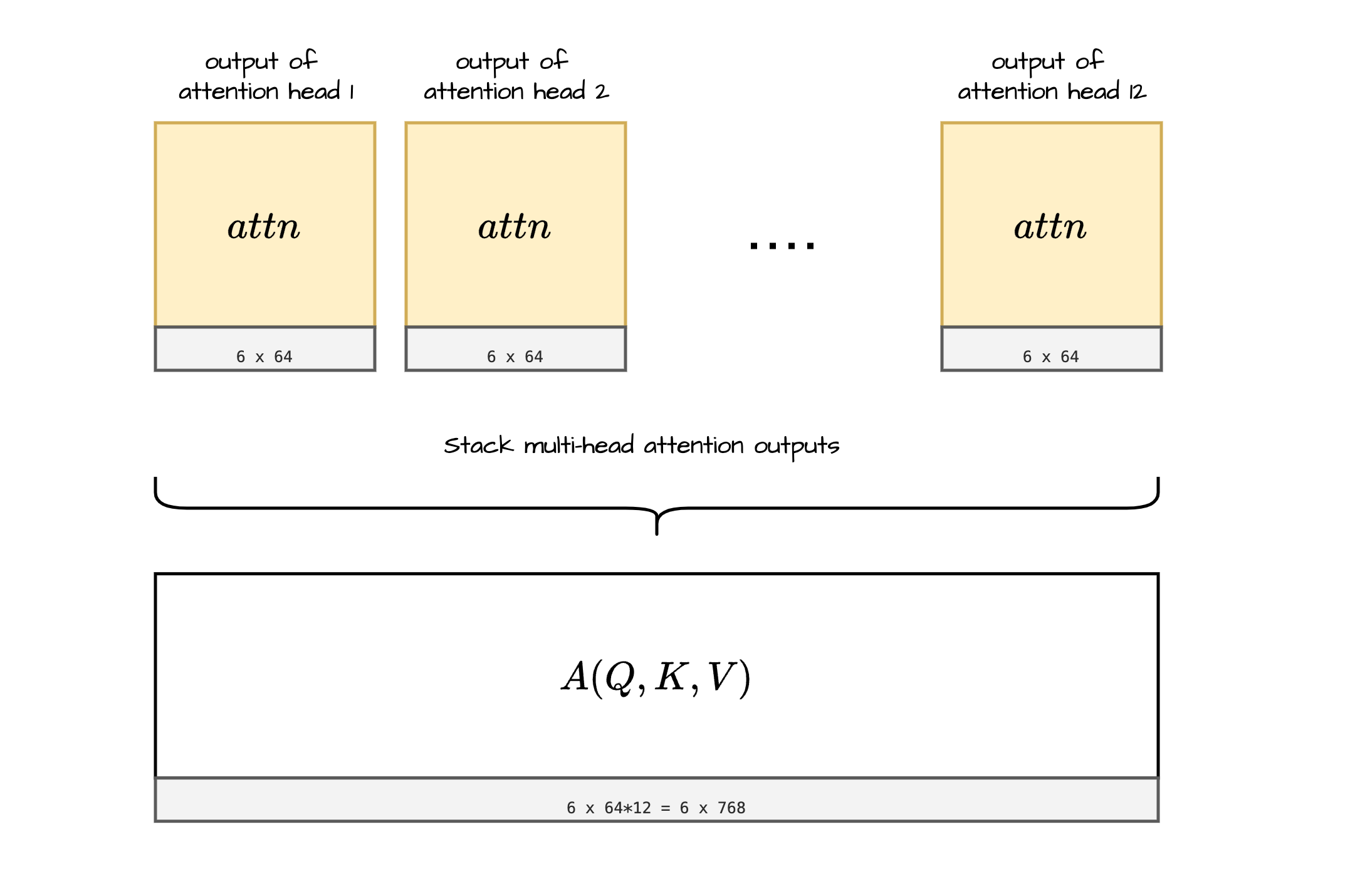
This further is multiplied by a projection matrix to get final output of Attention block.
Note on multi-head attention
In Step 3 we saw how single head attention works, now do the same across 12 parts of Q, K, V matrices, we have multi-head attention.
Now one might argue why do we not use the entire Q, K, V matrix instead of breaking it down into smaller pieces like shown above. Well here are few reasons for that:
- Feature Interaction:
- Each head can focus on different aspects of the input, allowing the model to capture various types of relationships and patterns simultaneously.
- This is similar to having multiple filters in CNNs, each detecting different features.
- Improved Representation and Robustness:
- Multiple heads allow the model to attend to information from different representation subspaces.
- This can lead to a richer and more nuanced overall representation of the input.
- Computational Efficiency:
- Parallel computation of smaller matrices can be more efficient than a single large matrix operation.
- This is particularly beneficial on GPU hardware optimized for parallel operations.
Outputs (Step 4)
In this step we get A(Q,K,V)* [6 x 768] output which we can finally call “final attention ouptut”, hush!
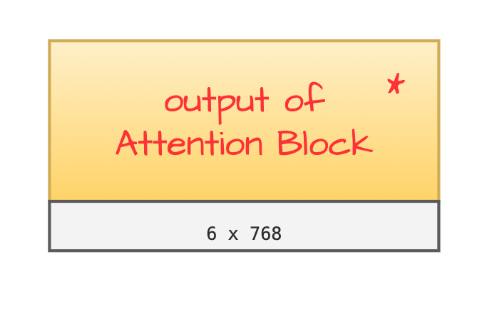
Output of Attention Block
NOTE - One important thing to notice here is the output of attention block is of the same shape that we began with [6 x 768].
Step 5 - MLP Block
Where are we now?
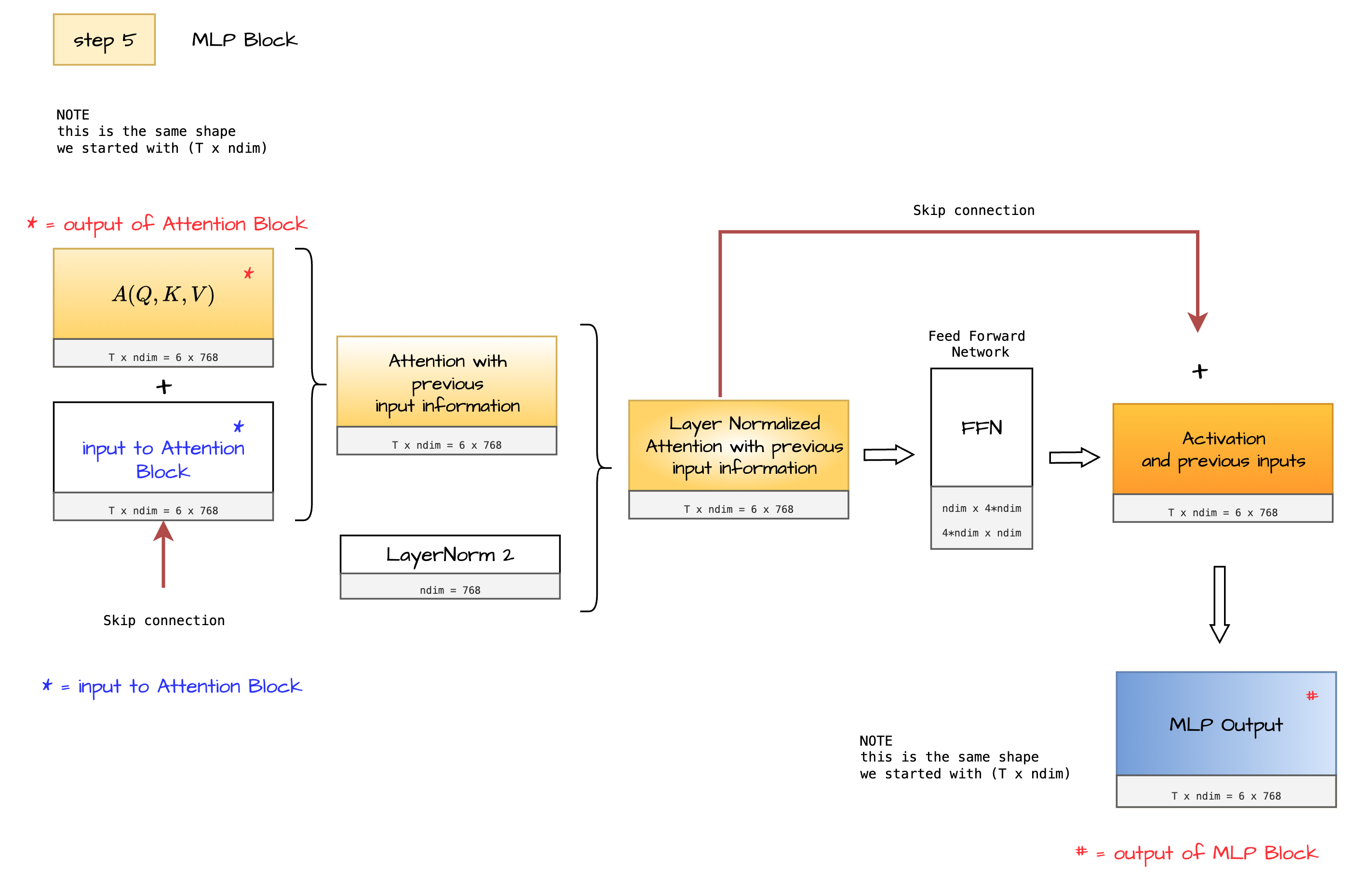
We have covered quite some ground now, we are currently at output of Attention Block it is important that you look at input to Attention Block as well, as both of these will be used in this step, it is the skip connection that enables usage of previous information.
Inputs (Step 5)
Output of Attention Block A(Q,K,V)* [6 x 768] serves as input to this MLP block.
Here both the inputs (here $x$) and outputs of Attention Block (here $Attention(x)$) are combined together using a skip connection as below. The Add and Norm block of decoder architecture can be given by this equation.
$$ y=LayerNorm(x+Attention(x)) $$
This intermediate output $y$ is further passed through feed forward network and is added with output of feed forward network through another skip connection. This can be better understood with the equation below.
$$ z=LayerNorm(y+FFN(y)) $$
This gives the output of MLP block # denoted by $z$ above, notice the shape of MLP block it is same shape that we started with [6 x 768], this shape enables us to further pass this $z$ back to the transformer. The small Nx in the diagram denotes repetion of the Attention and MLP block block (hidden module) as shown below.
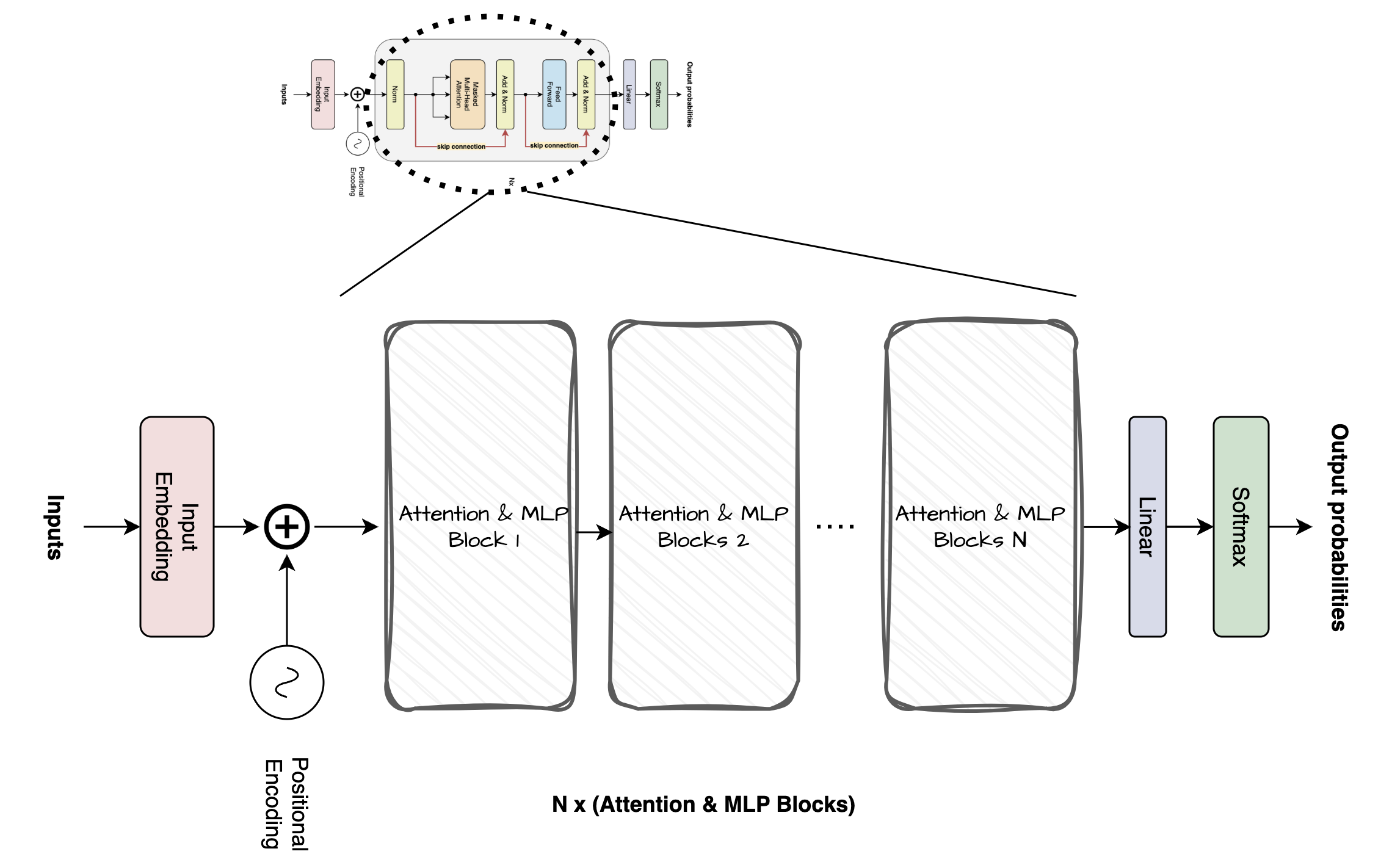
Expanded Attention and NLP block
Outputs (Step 5)
At the end of Attention and MLP blocks we get a matrix of shape [T x ndim] here [6 x 768].
Step 6 - LM head
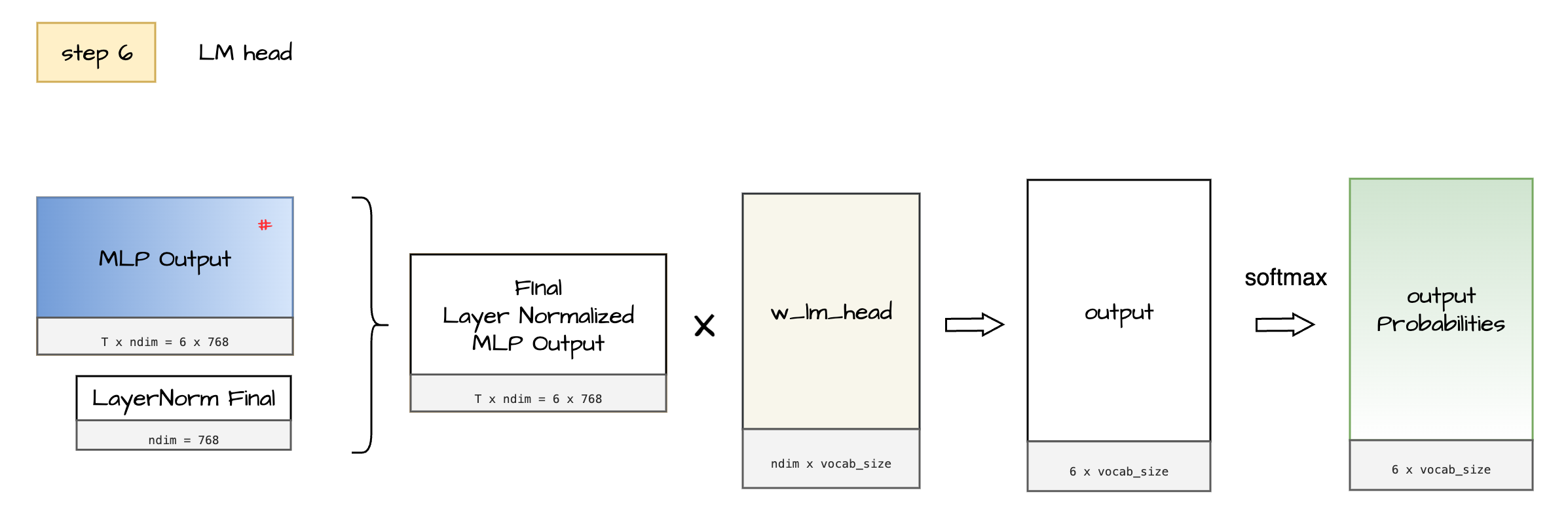
In this step we look at final transformations to generate output probabilities.
Inputs (Step 6)
Outputs of hidden layers - N x (Attention and MLP blocks) serve as input to this step.
Process
MLP Output goes through another projection here to get output which holds logits before they are converted into final probability scores. Each row of the in matrix [6 x 768] is probability distribution of which words are most likely to come next in the sequence. We can interpret the final output as follows.
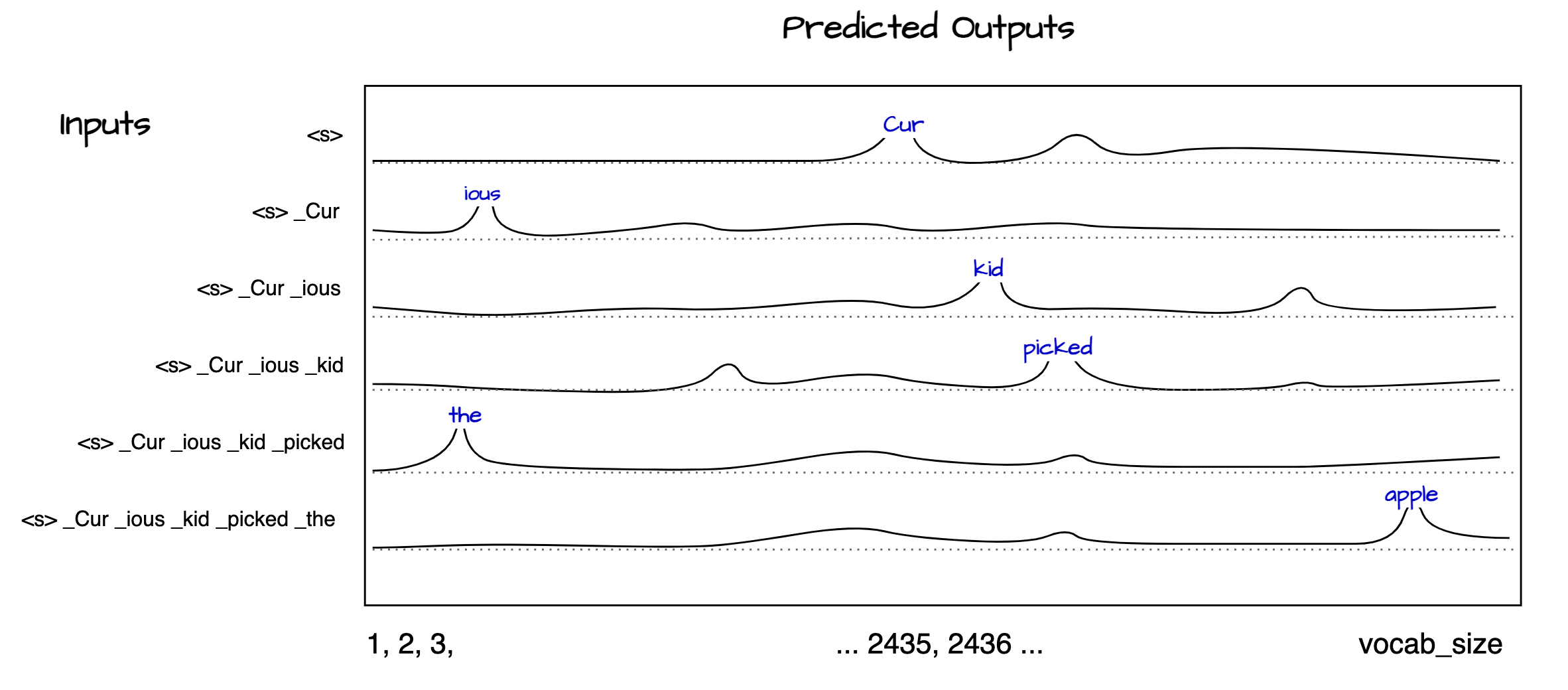
Softmax and output probabilities while training
Ouptut
The output of this step is a set of probabilities with dimensions [T x ndim], which in this case is [6 x 768]. During the training phase, these probabilities are compared with the target matrix to compute the loss. It’s important to note that all subsequent tokens are predicted simultaneously during training.
During inference, we do not know the next token in advance. Therefore, we must generate each token one at a time, waiting for the model to predict each subsequent token until it outputs an end-of-sequence token. This sequential generation continues until the model indicates that the sequence is complete.
End note
This brings us to the end of a deep dive into transformers and its components. I hope this blog has provided you with a solid understanding and inspired you to delve deeper into concepts.
Happy learning!
References
- Intuition behind encoder and attention mechanism by - Erik Storrs
- Attention Is All You Need: Discovering the Transformer Paper
- Transformers Explained Visually (Part 3): Multi-Head Attention Deep Dive
- The Illustrated Transformer by Jay Alammar
- University of Waterloo Lecture: Attention and Transformers
- Serrano Academy
- Attention Visualized by Umar Jamil
- Decoder Only Transformer architecture
- LayerNorm explained
- Layer Normalization Pinecone
- Illustrated GPT-2
Almost all diagrams were drawn on draw.io and few edits on canva.com, feel free to use these diagrams with credits.

