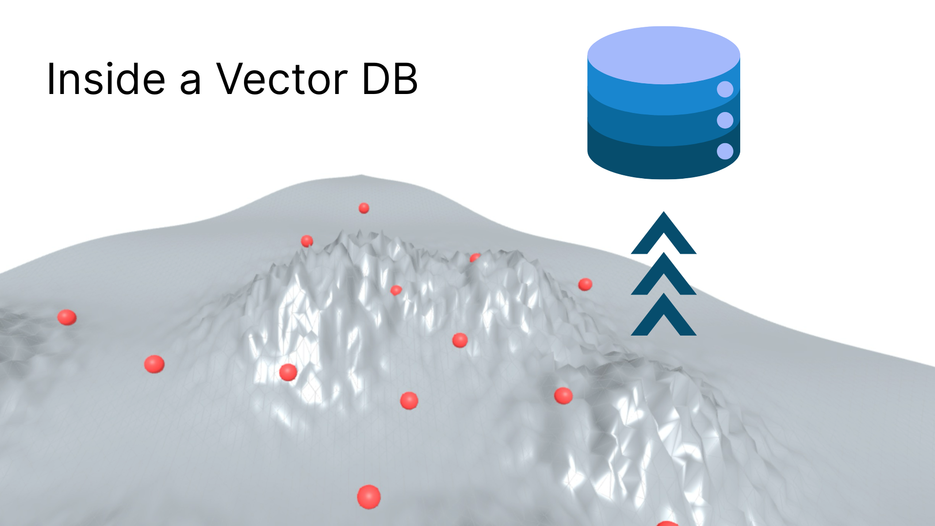
Introduction
Imagine you are an e-commerce platform with say 10 million products on your website. Your customers are searching for products by name, description, or attributes. You want the ability to find the products that are most similar to the query. How do you go about it? Fuzzy searches / Keyword searches, well it would fail miserably given the scale and nature of the problem.
When keyword search is insufficient, we need semantic search powered by vector similarity! Product descriptions can be encoded as vectors using embeddings, but how do we store these vectors and query them efficiently at scale? This is where VectorDBs come into play.
Traditional route
When we fire a query to a traditional database, it is a simple table lookup. But here your natural language query is encoded to an n-dimensional vector first and then looked up in the database holding more such vectors.
This is where the magic happens: Vector Similarity Search.
The Brute Force Problem
The most straightforward approach to find similar vectors is the K-Nearest Neighbors (KNN) exact search. Here’s how it works:
- Take your query vector
- Compare it with every single vector in the database
- Calculate distance (cosine, euclidean, etc.) for each comparison
- Sort all distances and return the K closest vectors
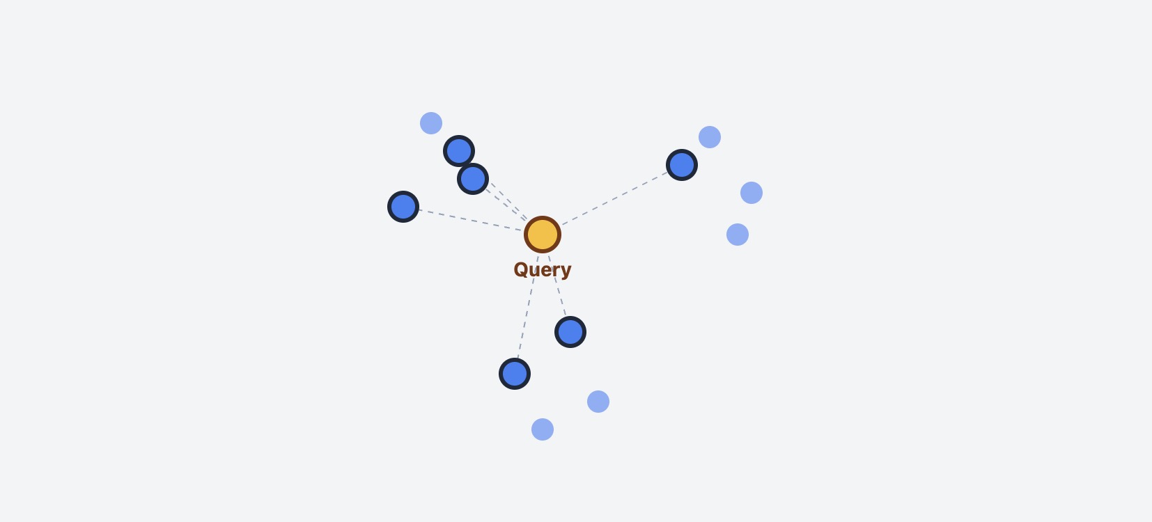
KNN exact search: Query vector compared against all N vectors in database
Why This Doesn’t Scale
Let’s put this into perspective with some numbers:
- Database size: 10 million product vectors
- Vector dimensions: 768 (typical for text embeddings)
- Query time: For each search, you need 10M distance calculations
- Memory: Vectors are typically memory-mapped or batched for efficient access
All this with additional overhead of doing cosine similarity calculation which itself is a computationally intensive operation and increases with dimensionality of the vectors.
1# Pseudo-code for brute force search
2def knn_search(query_vector, database_vectors, k=5):
3    distances = []
4    for vector in database_vectors:  # O(N) - This is the problem!
5        distance = calculate_distance(query_vector, vector)
6        distances.append((distance, vector))
7
8    # Sort and return top K
9    return sorted(distances)[:k]  # O(N log N)
The time complexity is O(N) for each query, where N is the number of vectors. With millions of vectors and hundreds of concurrent users, this becomes computationally prohibitive.
Real-world impact:
- Query latency: Several seconds per search
- CPU usage: Maxed out with just a few concurrent users
- Memory requirements: Entire dataset must fit in RAM
- Cost: Expensive hardware for acceptable performance
Can we do better than this?
The smarter route
Instead of going through all the vectors, we can utilize inherent nature of the vectors to our advantage. Can we skip some of the vectors and still get approximate neighbors without losing relevance? Turns out we can, if we use clever data structures to store these vectors.
Here are some approaches to get approximate nearest neighbors:
- KD Trees
- Locality Sensitive Hashing (LSH)
- Annoy
- HNSW
We will focus on HNSW in detail to keep the scope brief, it is widely used in practice across industry.
Textbook description of HNSW
HNSW stands for Hierarchical Navigable Small World, a powerful algorithm for performing approximate nearest neighbor (ANN) searches in high-dimensional vector spaces. It organizes data into a multi-layered, hierarchical graph structure, allowing for very fast similarity searches by using long-range “skip” connections in upper layers to quickly narrow down the search area, and fine-grained searches in lower layers to find the most accurate results.
Too many words!
Real World Travel Analogy
Imagine you live in a city in state $S_1$ and want to visit a remote village in state $S_k$. Instead of driving through every town, you use the hierarchical highway system:
Level 2 - Interstate Roads (State-to-State)
Goal: navigate from one state to another.
- States ($S_1$, $S_2$, $S_k$): Represent major regions in the vector space
- Solid arrows: Direct interstate highways between states
- Dashed arrows: Long-distance connections that can be skipped
- Navigate from $S_1$ -> $S_2$ … -> $S_k$ using the most efficient interstate route
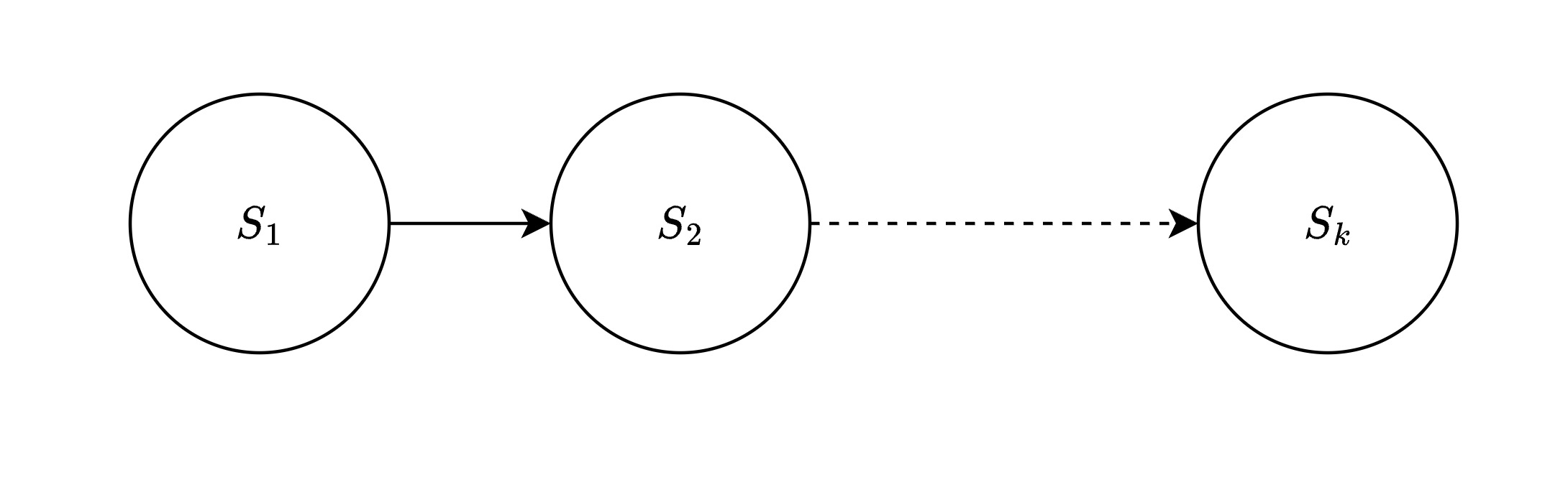
Level 2: State-to-State travel using Interstate roads
Level 1 - Regional Travel (Inter-City)
Goal: navigate through cities.
- Gray circles: Regular cities/vectors within each state
- Red circles: Hub cities that connect to other states
- Hatched areas: Irrelevant regions skipped during greedy search
- Blue circle: Target destination in state $S_k$
- Search within the relevant regions, skip irrelevant areas
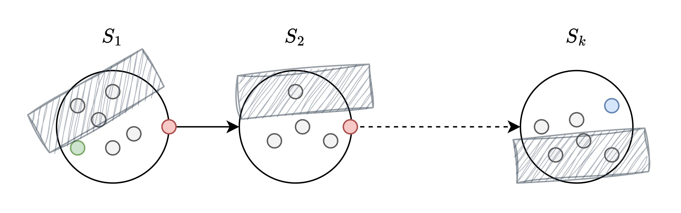
Level 1: Inter-city travel within states
Level 0 - Local Navigation (Village-to-Village)
Goal: navigate through villages.
- Connected nodes: Local road networks between nearby cities
- Green path: Actual search route taken from start to target
- Blue dotted connections: Final local connections to reach destination
- Navigate through local connections to find the exact target vector
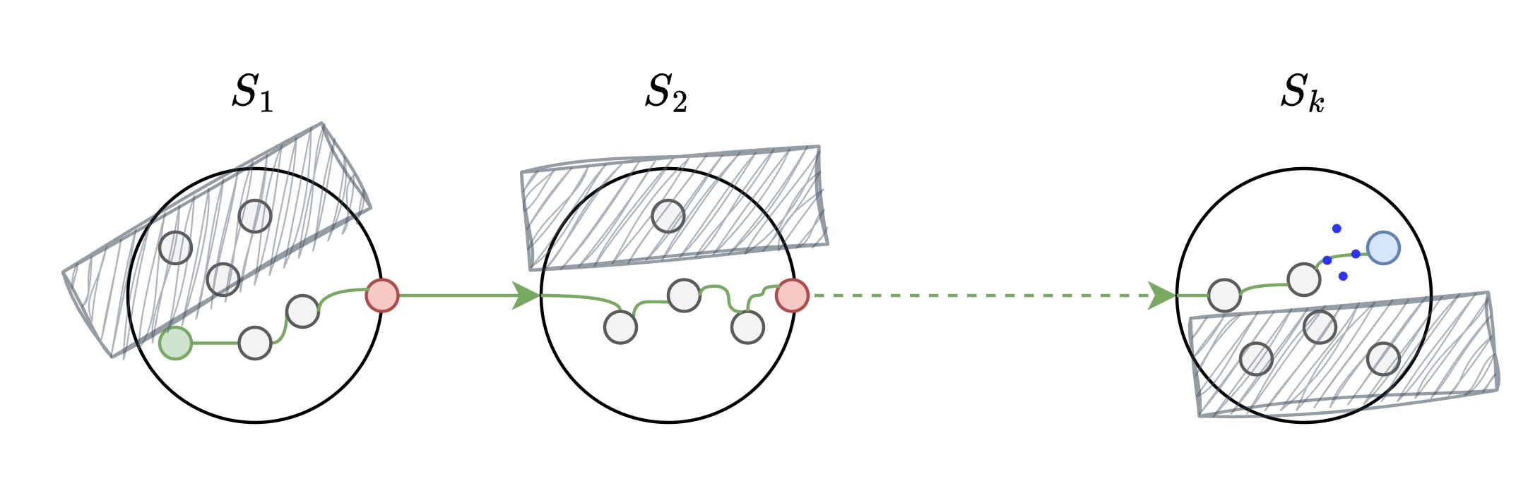
Level 0: Village-to-village local navigation
Why This Works
- Hub Cities: Act as shortcuts connecting distant regions efficiently
- Hierarchical Levels: Each level provides different granularity of navigation
- Skip Irrelevant Areas: Never waste time in regions that don’t help
- Approximate Results: Fast navigation to very good destinations
This is exactly how HNSW manages to find approximate nearest neighbors - using smart way of organizing vectors, similarity search can be optimized for speed while still maintaining relevance.
How HNSW works
Here we will dive deep into internals of how HNSW works.
Skip lists and HNSW
In order to simulate “skipping of vectors” we use a special data structure like skip list. This enables us to skip some of the vectors and still get approximate nearest neighbors.
Visualization of a skip list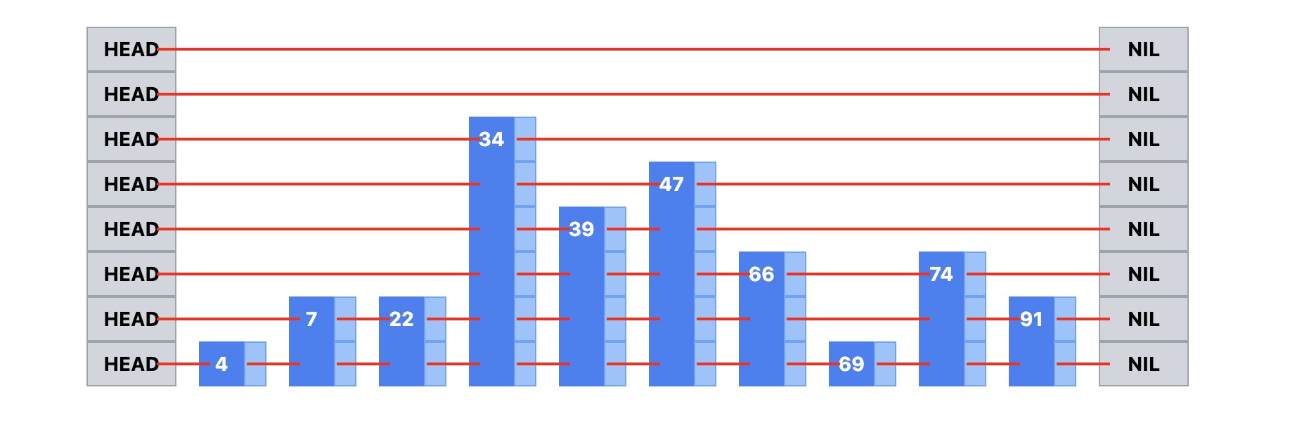
- Bottom level: All nodes (4, 7, 22, 34, 39, 47, 66, 69, 74, 91)
- Higher levels: Progressively fewer “hub” nodes (34, 47, 74 at top)
- Search path: Start from HEAD, use express lanes, drop down when needed
Here are some properties of a skip list that align very well with HNSW:
- Multi-level indexing: Higher levels contain fewer nodes for faster traversal
- Logarithmic search: O(log n) search time instead of O(n) linear search
- Express lanes: Upper levels act like highways to jump across large distances
- Progressive refinement: Start high, drop down levels to get more precise
- Probabilistic structure: Nodes randomly promoted to higher levels
- Efficient skipping: Can bypass many irrelevant nodes during search
The same skip list can be represented as a graph as shown below: Equivalent graph representation of a skip list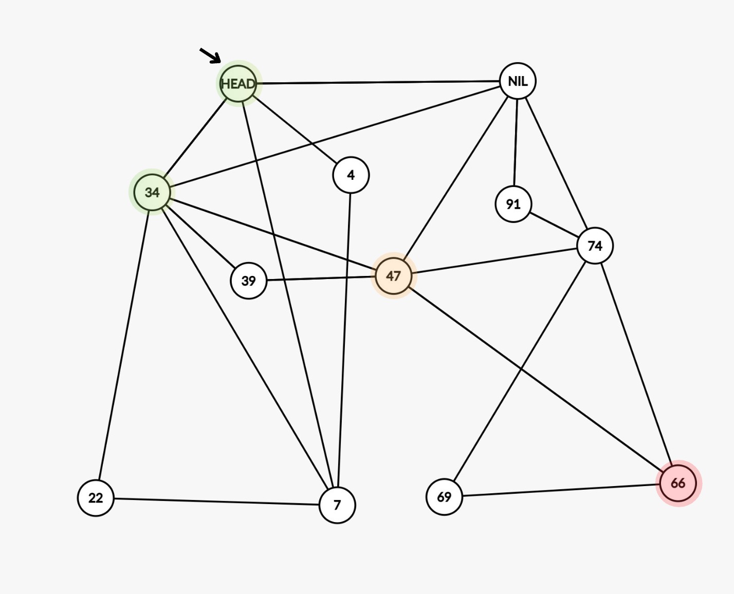
Notice: In order to find 66, (HEAD -> 34 -> 47 -> 66) you jump through just 2 nodes, this is the power of skip list.
Core Algorithm of HNSW (Simplified)
Level assignment
What does it mean when we say level of vector A is 2?
- A vector can exist on multiple levels simultaneously: 0, 1, and 2
- Think of it like an employee who has access to level 2 clearance - they also have access to all levels below it (1 and 0)
- By default, every vector is present in level 0
How is this level assigned?
- Level is assigned using an exponential-like distribution
- Formula:
max_level = floor(-ln(U) * mL)where:U ~ uniform(0,1)is a random numbermL = 1/ln(M)is the level multiplier (normalization factor)
- The formula
floor(-ln(U) / ln(M))is equivalent but shows the dependency on M directly - Some implementations allow tuning
mLindependently to control hierarchy height
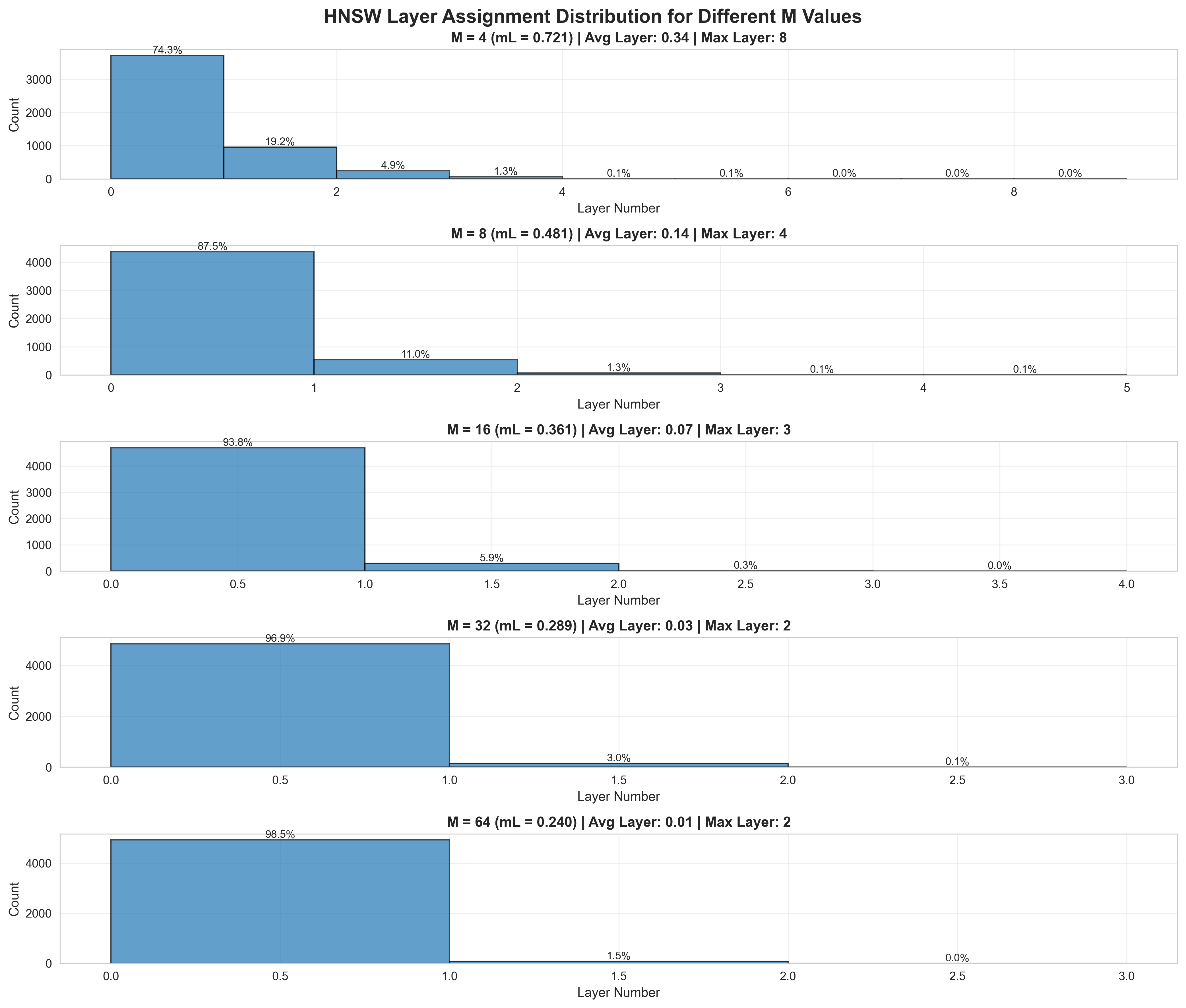
Distribution of levels in HNSW
Why is exponential-like distribution used?
- It naturally favors lower levels - most vectors exist only at L=0
- Very few vectors exist at higher levels (exponentially decaying probability)
- Sampling from this distribution ensures hierarchical structure similar to skip lists
- Setting
mL = 0would create a single-layer graph (no hierarchy)
Close friends
- In a social setting, you have a few close friends that you regularly hang out with
- HNSW also likes to follow this pattern
- Each vector is allowed to keep
Mnumber of close friends - Close friends = Nearest neighbors
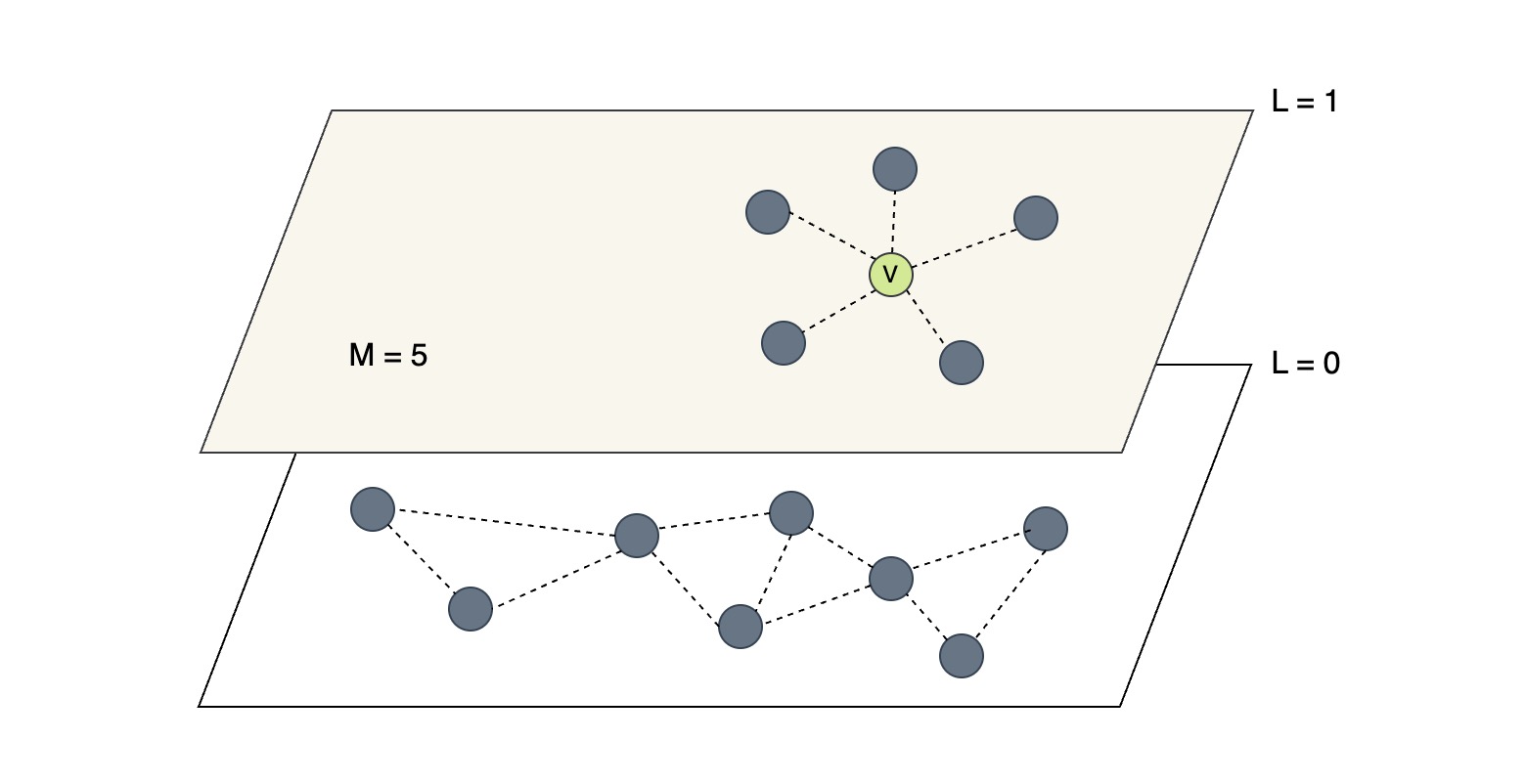
Vector V has M=5 neighbors per node
- Dotted lines represent bidirectional edges between vectors
- Note on bidirectionality: When vector V connects to neighbor N, N must also add V to its neighbor list. If N already has M neighbors, it must prune one neighbor to stay within the limit (potentially V itself if V is the furthest). After pruning, edges are not guaranteed to be perfectly symmetric across the graph.
New person in the town
- When a new person arrives in town, they don’t randomly knock on every door they get an introduction and explore the social network through connections
- Similarly, inserting a new vector means navigating the graph through existing connections to find the best neighbors
When inserting a new vector into HNSW, the algorithm doesn’t scan all existing vectors. Instead, it uses a greedy search process starting from an entry point:
The insertion process:
K candidates"] connect["Connect
Best M neighbors"] newVector --> search search --> connect style newVector fill:#E3F2FD,stroke:#1976D2,stroke-width:3px style search fill:#E8F5E9,stroke:#388E3C,stroke-width:3px style connect fill:#FFEBEE,stroke:#D32F2F,stroke-width:3px
Step-by-step breakdown:
- Entry point: Start from the entry point provided by the layer above
- Greedy search: Navigate through the graph by examining neighbors of the current node, always moving to the neighbor closest to the new vector
- Candidate pool: During this search, maintain a list of the K closest vectors encountered (these are potential neighbors)
- Edge creation: From this candidate pool, select the top M closest vectors and create bidirectional edges to them
Why K > M?
- K controls the search breadth during insertion. A larger value means exploring more candidates before selecting neighbors
- M limits the number of edges per node, keeping the graph’s connectivity manageable
- By evaluating K candidates (e.g., 100) but only connecting to M neighbors (e.g., 16), we get better quality connections while maintaining efficient graph structure
Parameter naming clarification:
- During construction: The parameter K is called
efConstruction- it controls how many candidates to evaluate when inserting a new vector- During search/query: The parameter is called
ef(oref_search) - it controls how many candidates to evaluate when searching for neighbors- Both control exploration breadth, but affect different phases (build time vs query time)
Key insight: K > M
- Larger K -> better neighbor selection (higher recall)
- Smaller M -> fewer edges per node (faster queries, lower memory)
Mutual Friends: The Bridge Between Circles
- When you want to meet someone from a distant social circle, you don’t randomly reach out you find a mutual friend who bridges both groups
- HNSW uses the same idea: routing nodes are vectors that bridge distant regions of the vector space
Example: Vector Q gets assigned Level = 2
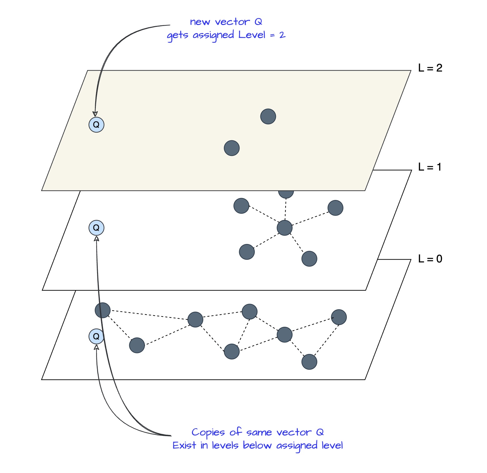
Vector Q exists on multiple levels after being assigned max_level = 2
When new vector Q is inserted and gets assigned Level = 2:
- Q exists on L=2, L=1, and L=0: Same vector, but “copies” appear at each level in the hierarchy
- At each level, Q searches for and connects to different nearest neighbors:
- At L=2: Q finds its nearest neighbors among the ~3 vectors at L=2 (sparse, long-range connections)
- At L=1: Q finds its nearest neighbors among the larger set at L=1 (medium-range connections)
- At L=0: Q finds its nearest neighbors among ALL vectors at L=0 (dense, short-range connections)
Why multi-level neighbors solve the reachability problem:
- At L=0 alone: Each node limited to M neighbors means limited connectivity. Some vectors may be unreachable through the existing neighbor connections
- At L=2: With only ~3 vectors total, Q’s M neighbors provide connections to much broader regions of the vector space
- The hierarchy improves graph connectivity: L=2 provides global connectivity, L=1 provides regional connectivity, L=0 provides local precision
The bridging property emerges from scarcity:
- Fewer routing nodes at higher levels: L=2 has only 3 vectors -> Q’s M neighbors span broader regions, creating bridges to otherwise disconnected parts of the graph
- More routing nodes at lower levels: L=0 has all vectors -> Q’s M neighbors connect to nearby nodes, providing local precision
- Hierarchical navigation: Start at Q on L=2 (reach different regions), descend to Q on L=1 (refine), finally Q on L=0 (find precise neighbors)
Key insight: Q having different neighbors at each level enables efficient graph traversal. At L=0, M neighbors provide local connectivity. At L=2, those same M neighbor slots provide global connectivity across the vector space, solving reachability problems that plague single-level graphs.
Performance Tests: Brute Force vs HNSWlib vs FAISS
Now that we understand how HNSW works, let’s see how it performs in practice. I ran some tests on 1M documents from the MS MARCO dataset.
Important: These are exploratory tests, not rigorous benchmarks. Full experimental code and configurations are available here: https://github.com/sagarsrc/inside-vectordb
Experimental Setup
Dataset: MS MARCO (1M documents, 768-dimensional embeddings)
Methods:
- Brute Force: sklearn cosine similarity (baseline, 100% recall)
- HNSWlib: M=32, ef_construction=100, ef_search=50
- FAISS HNSW: M=32, ef_construction=100, ef_search=50
Distance Metric: Cosine similarity (implemented as L2-normalized inner product)
Results
Performance Summary
| Method | Implementation | Latency | Throughput | Recall@10 | Speedup |
|---|---|---|---|---|---|
| Brute Force | sklearn | 699.43 ms | 1.4 QPS | 0.8100 (100%) | 1x |
| HNSWlib | C++ with Python bindings | 0.46 ms | 2,166 QPS | 0.7433 (91.8%) | 1,515x |
| FAISS HNSW | IndexHNSWFlat | 0.08 ms | 11,805 QPS | 0.7683 (94.9%) | 8,257x |
NOTE: The numbers are inflated as we are using 384 dimension vectors, in practice dimensionality is much higher and would affect latency and throughputs.
Visual Comparisons
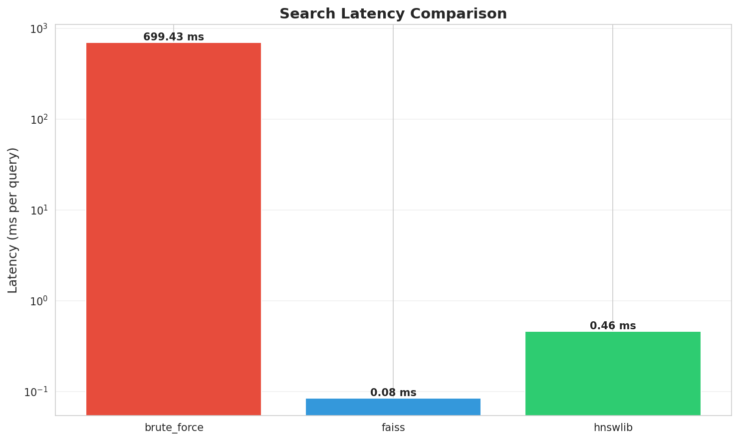
Latency comparison: FAISS achieves sub-millisecond queries
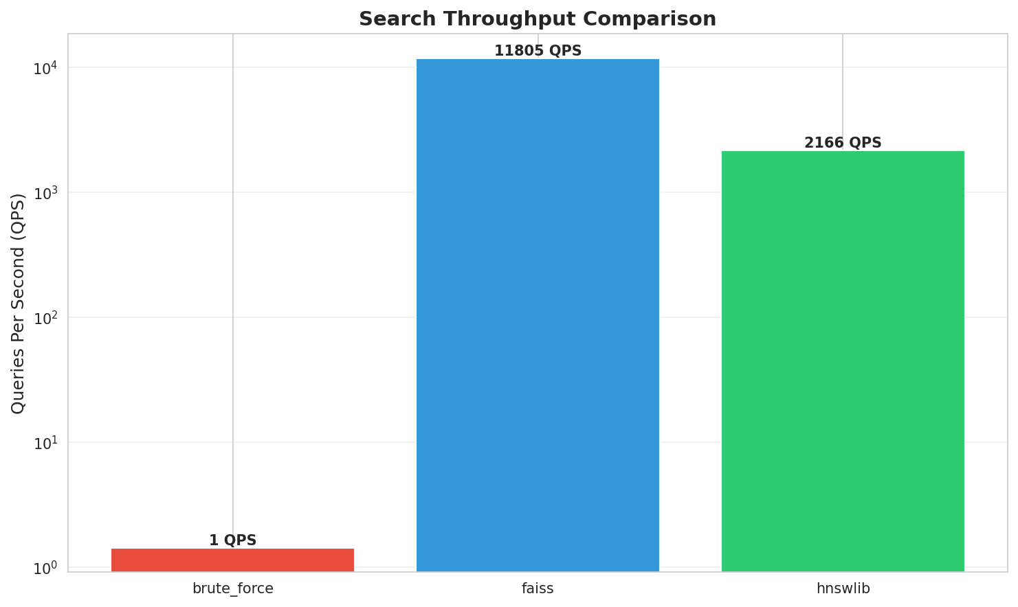
Throughput: FAISS processes 11,805 queries/second
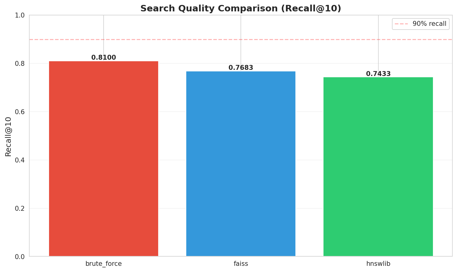
Recall@10: HNSW maintains 91.8-94.9% accuracy relative to brute force
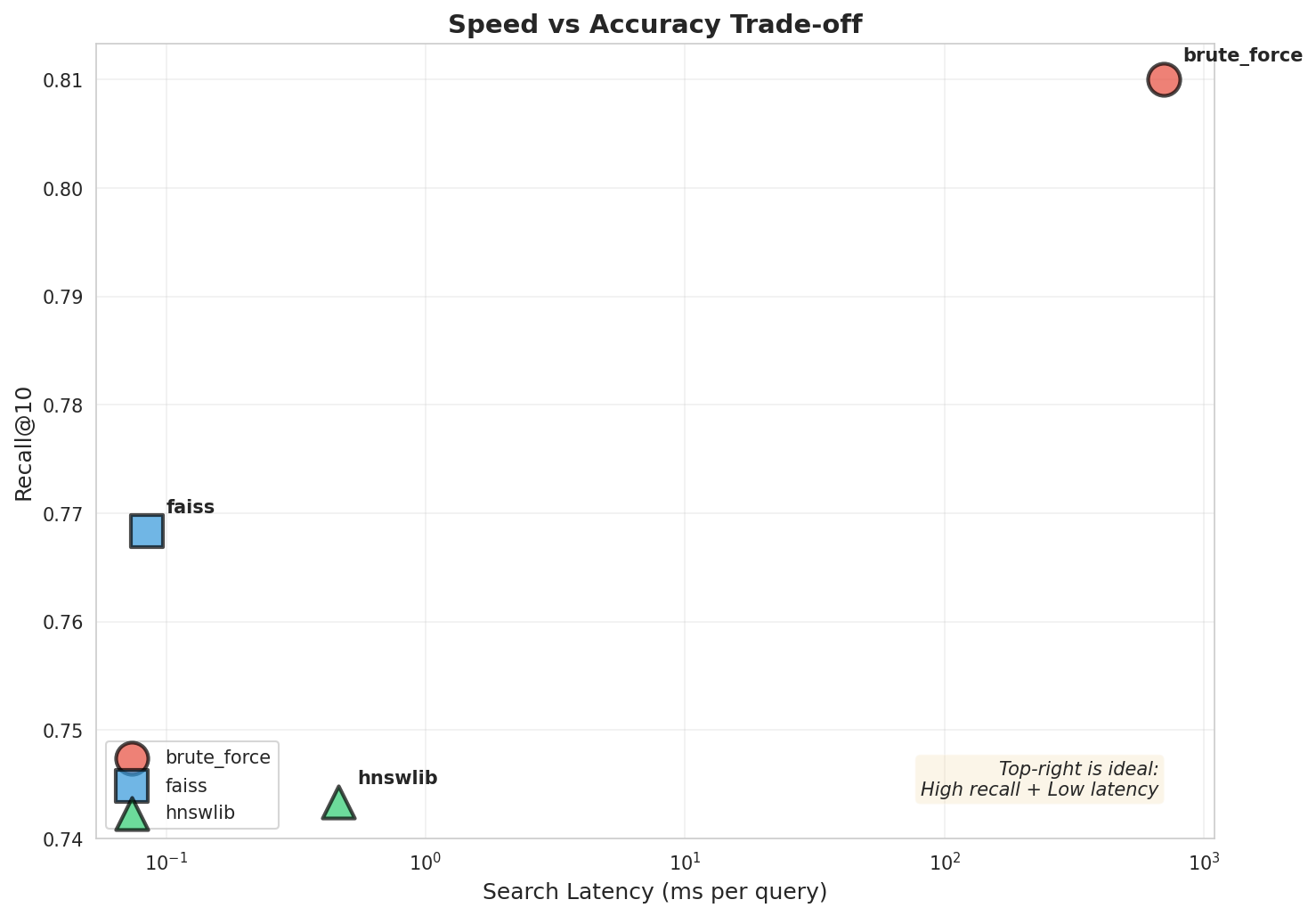
Speed vs Accuracy: 1500-8000x speedup with 5-8% recall loss
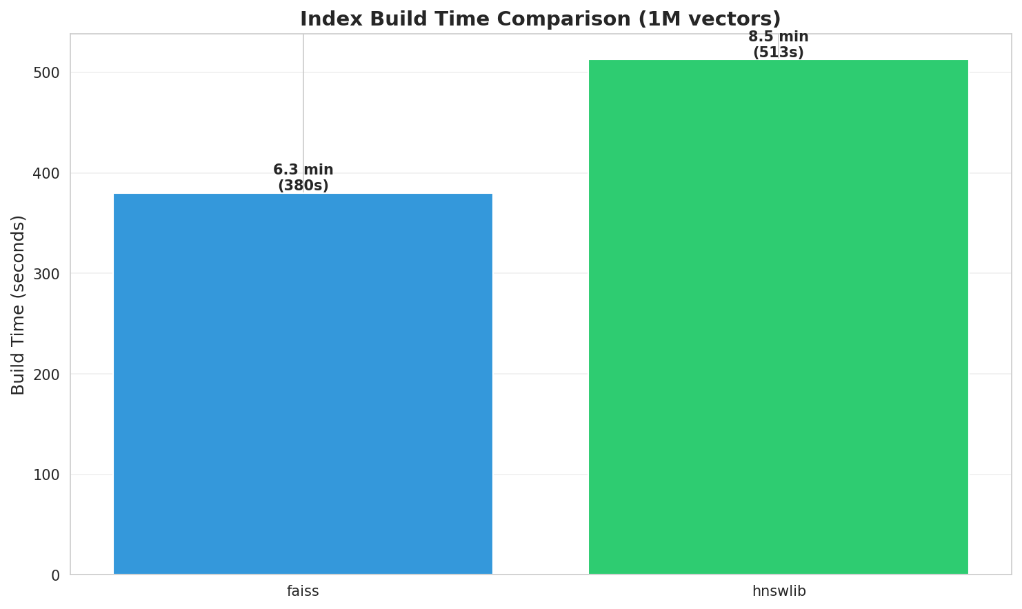
Build time comparison across methods
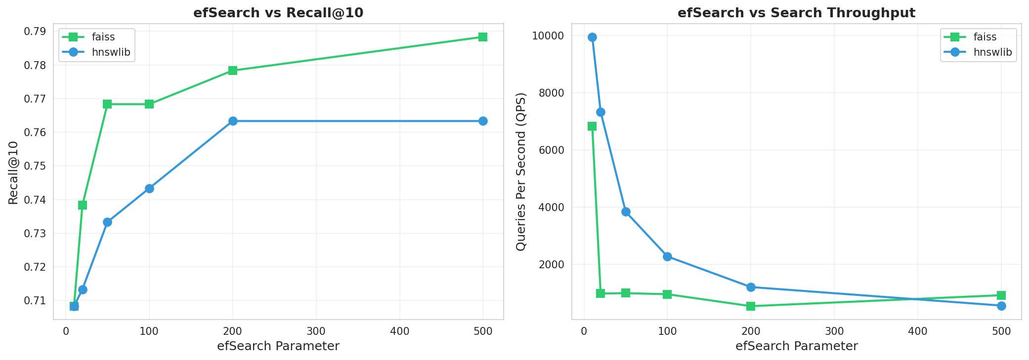
ef_search sensitivity analysis showing recall-latency tradeoffs
Key Observations
- HNSW delivers massive speedups: 1500-8000x faster than brute force, sacrificing only 5-8% recall
- Fair comparison: Both implementations use M=32, making this a true apples-to-apples comparison
- FAISS optimizations shine: FAISS’s highly optimized C++ implementation gives it 5x better throughput than HNSWlib
- Sub-millisecond queries at scale: Both HNSW methods achieve sub-millisecond latency on 1M vectors
- Recall-speed tradeoff: The ef_search parameter allows fine-tuning between recall and latency based on application needs
Closing Notes
Vector databases power modern AI from semantic search to RAG systems. HNSW’s clever hierarchical design makes searching millions of vectors feel instant.
Key insights:
- Skip list hierarchy creates express lanes through vector space
- Random level assignment naturally creates routing nodes
- Multi-level neighbors solve graph connectivity same vector, different connections at each level
- Parameters matter: M (memory), efConstruction (build quality), ef_search (query speed)
- Approximate wins: 94% recall with 1000x+ speedup
Full code and experiments on GitHub: https://github.com/sagarsrc/inside-vectordb
References
- Efficient and robust approximate nearest neighbor search using Hierarchical Navigable Small World graphs
- Getting started with HNSWlib
- FAISS IndexHNSW cpp code github
- Generate a random Skip list
- Graph Visualization of Skip list
- Redis and Parameters of HNSW
- Hierarchical Navigable Small Worlds (HNSW) by Pinecone